Lesson 5 Continuous Probability Distributions Kafu Wong 2004

Outline Continuous probability distributions Features of univariate probability distribution Features of bivariate probability distribution Marginal density and Conditional density Expectation, Variance, Covariance and Correlation Coefficient Importance of normal distribution The normal approximation to the binomial Ka-fu Wong © 2004 ECON 1003: Analysis of Economic Data 2

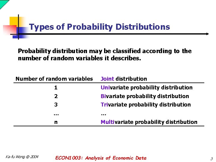
Types of Probability Distributions Probability distribution may be classified according to the number of random variables it describes. Number of random variables Ka-fu Wong © 2004 Joint distribution 1 Univariate probability distribution 2 Bivariate probability distribution 3 Trivariate probability distribution … … n Multivariate probability distribution ECON 1003: Analysis of Economic Data 3

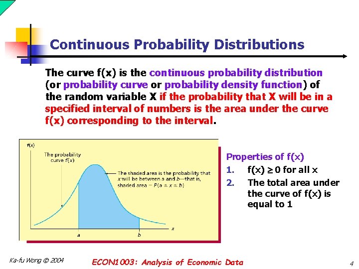
Continuous Probability Distributions The curve f(x) is the continuous probability distribution (or probability curve or probability density function) of the random variable X if the probability that X will be in a specified interval of numbers is the area under the curve f(x) corresponding to the interval. Properties of f(x) 1. f(x) 0 for all x 2. The total area under the curve of f(x) is equal to 1 Ka-fu Wong © 2004 ECON 1003: Analysis of Economic Data 4

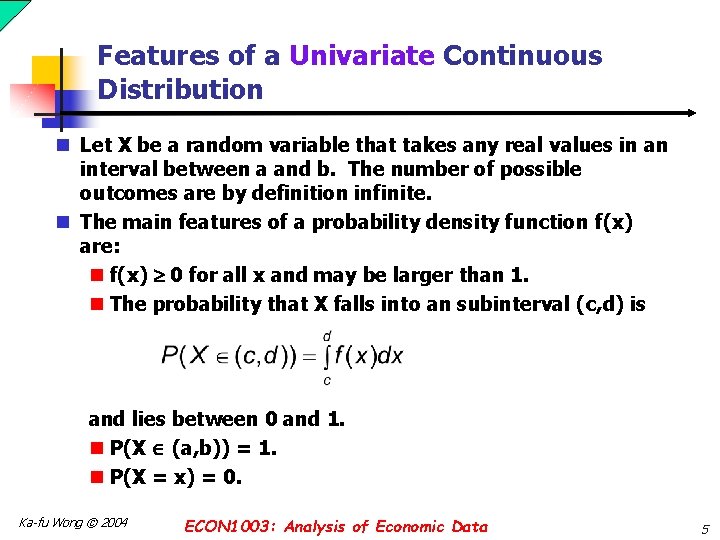
Features of a Univariate Continuous Distribution n Let X be a random variable that takes any real values in an interval between a and b. The number of possible outcomes are by definition infinite. n The main features of a probability density function f(x) are: n f(x) 0 for all x and may be larger than 1. n The probability that X falls into an subinterval (c, d) is and lies between 0 and 1. n P(X (a, b)) = 1. n P(X = x) = 0. Ka-fu Wong © 2004 ECON 1003: Analysis of Economic Data 5

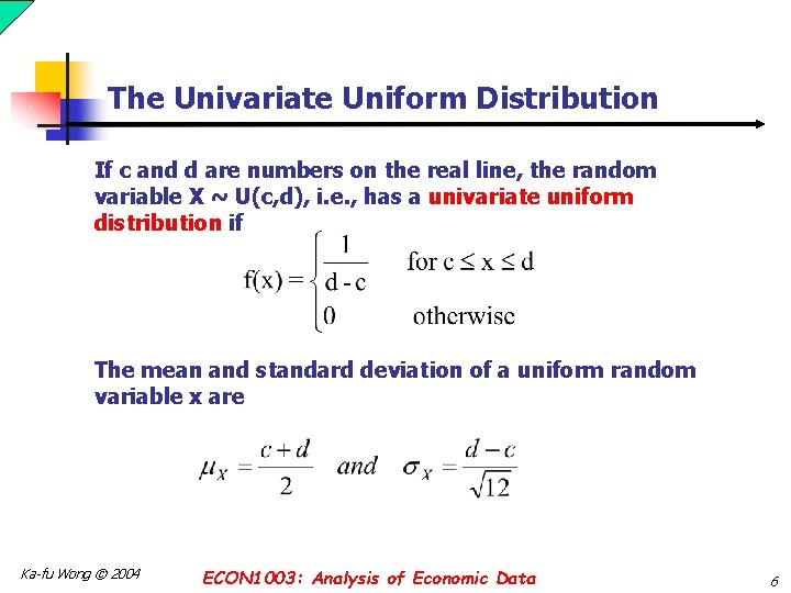
The Univariate Uniform Distribution If c and d are numbers on the real line, the random variable X ~ U(c, d), i. e. , has a univariate uniform distribution if The mean and standard deviation of a uniform random variable x are Ka-fu Wong © 2004 ECON 1003: Analysis of Economic Data 6

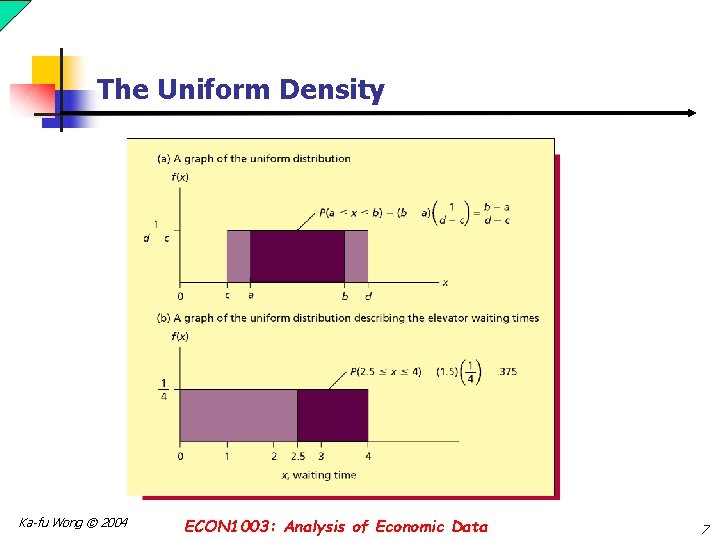
The Uniform Density Ka-fu Wong © 2004 ECON 1003: Analysis of Economic Data 7

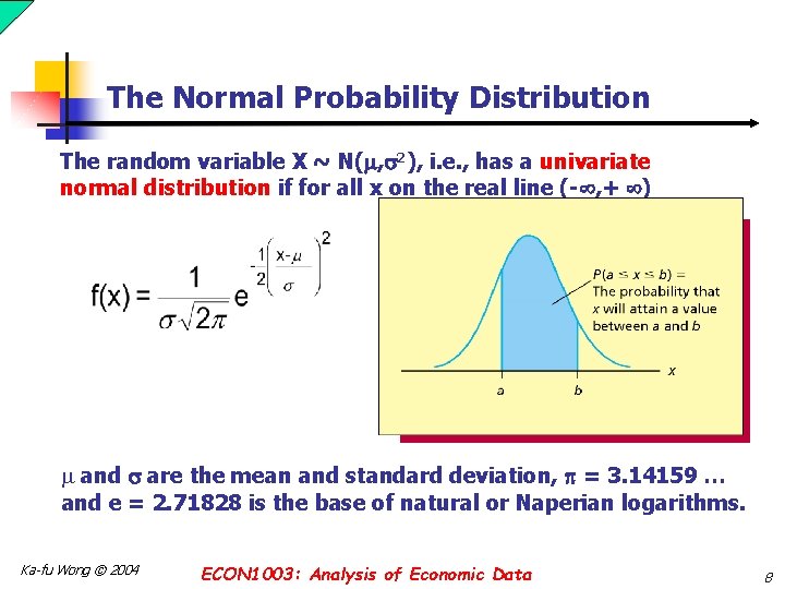
The Normal Probability Distribution The random variable X ~ N( , 2), i. e. , has a univariate normal distribution if for all x on the real line (- , + ) and are the mean and standard deviation, = 3. 14159 … and e = 2. 71828 is the base of natural or Naperian logarithms. Ka-fu Wong © 2004 ECON 1003: Analysis of Economic Data 8

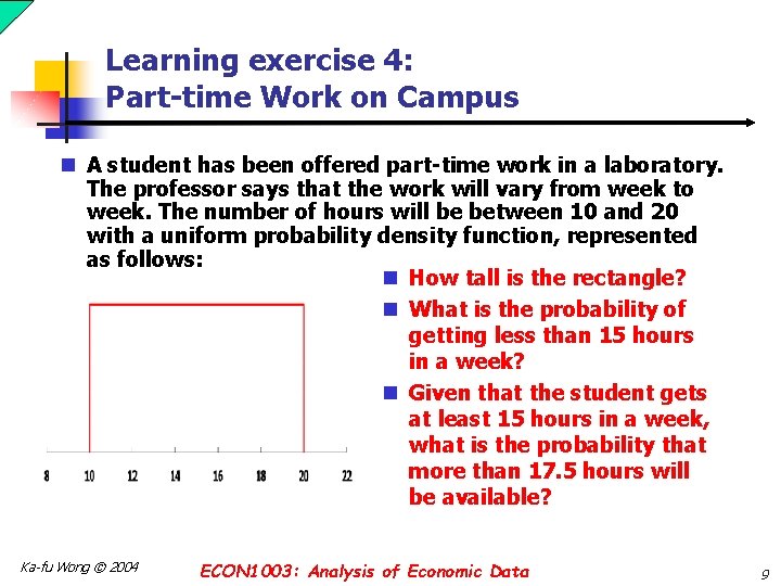
Learning exercise 4: Part-time Work on Campus n A student has been offered part-time work in a laboratory. The professor says that the work will vary from week to week. The number of hours will be between 10 and 20 with a uniform probability density function, represented as follows: n How tall is the rectangle? n What is the probability of getting less than 15 hours in a week? n Given that the student gets at least 15 hours in a week, what is the probability that more than 17. 5 hours will be available? Ka-fu Wong © 2004 ECON 1003: Analysis of Economic Data 9

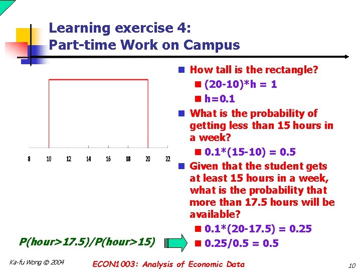
Learning exercise 4: Part-time Work on Campus P(hour>17. 5)/P(hour>15) Ka-fu Wong © 2004 n How tall is the rectangle? n (20 -10)*h = 1 n h=0. 1 n What is the probability of getting less than 15 hours in a week? n 0. 1*(15 -10) = 0. 5 n Given that the student gets at least 15 hours in a week, what is the probability that more than 17. 5 hours will be available? n 0. 1*(20 -17. 5) = 0. 25 n 0. 25/0. 5 = 0. 5 ECON 1003: Analysis of Economic Data 10

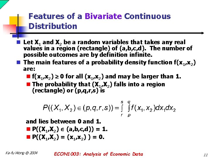
Features of a Bivariate Continuous Distribution n Let X 1 and X 2 be a random variables that takes any real values in a region (rectangle) of (a, b, c, d). The number of possible outcomes are by definition infinite. n The main features of a probability density function f(x 1, x 2) are: n f(x 1, x 2) 0 for all (x 1, x 2) and may be larger than 1. n The probability that (X 1, X 2) falls into a region (rectangle) or (p, q, r, s) is and lies between 0 and 1. n P((X 1, X 2) (a, b, c, d)) = 1. n P((X 1, X 2) = (x 1, x 2) ) = 0. Ka-fu Wong © 2004 ECON 1003: Analysis of Economic Data 11

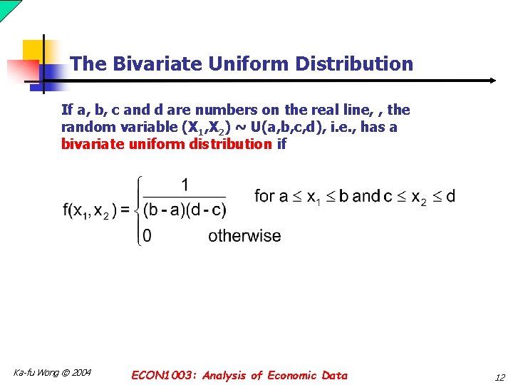
The Bivariate Uniform Distribution If a, b, c and d are numbers on the real line, , the random variable (X 1, X 2) ~ U(a, b, c, d), i. e. , has a bivariate uniform distribution if Ka-fu Wong © 2004 ECON 1003: Analysis of Economic Data 12

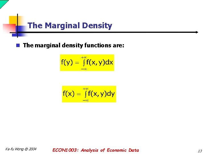
The Marginal Density n The marginal density functions are: Ka-fu Wong © 2004 ECON

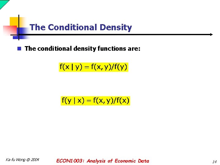
The Conditional Density n The conditional density functions are: Ka-fu Wong © 2004 ECON

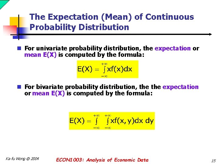
The Expectation (Mean) of Continuous Probability Distribution n For univariate probability distribution, the expectation or mean E(X) is computed by the formula: n For bivariate probability distribution, the expectation or mean E(X) is computed by the formula: Ka-fu Wong © 2004 ECON 1003: Analysis of Economic Data 15

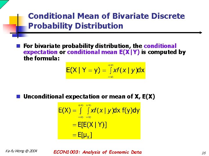
Conditional Mean of Bivariate Discrete Probability Distribution n For bivariate probability distribution, the conditional expectation or conditional mean E(X|Y) is computed by the formula: n Unconditional expectation or mean of X, E(X) Ka-fu Wong © 2004 ECON 1003: Analysis of Economic Data 16

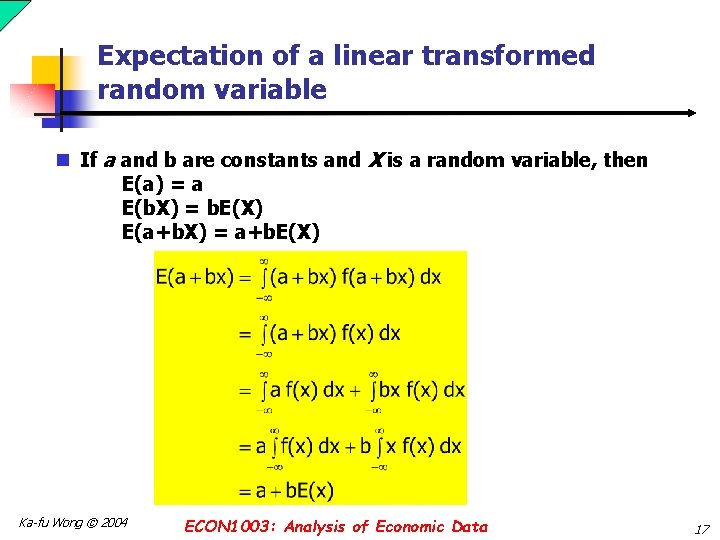
Expectation of a linear transformed random variable n If a and b are constants and X is a random variable, then E(a) = a E(b. X) = b. E(X) E(a+b. X) = a+b. E(X) Ka-fu Wong © 2004 ECON 1003: Analysis of Economic Data 17

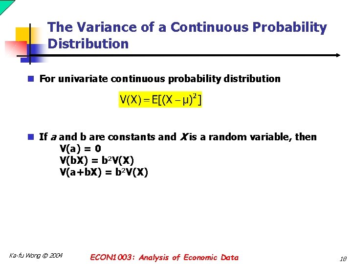
The Variance of a Continuous Probability Distribution n For univariate continuous probability distribution n If a and b are constants and X is a random variable, then V(a) = 0 V(b. X) = b 2 V(X) V(a+b. X) = b 2 V(X) Ka-fu Wong © 2004 ECON 1003: Analysis of Economic Data 18

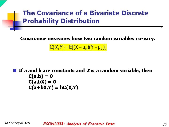
The Covariance of a Bivariate Discrete Probability Distribution Covariance measures how two random variables co-vary. n If a and b are constants and X is a random variable, then C(a, b) = 0 C(a, b. X) = 0 C(a+b. X, Y) = b. C(X, Y) Ka-fu Wong © 2004 ECON 1003: Analysis of Economic Data 19

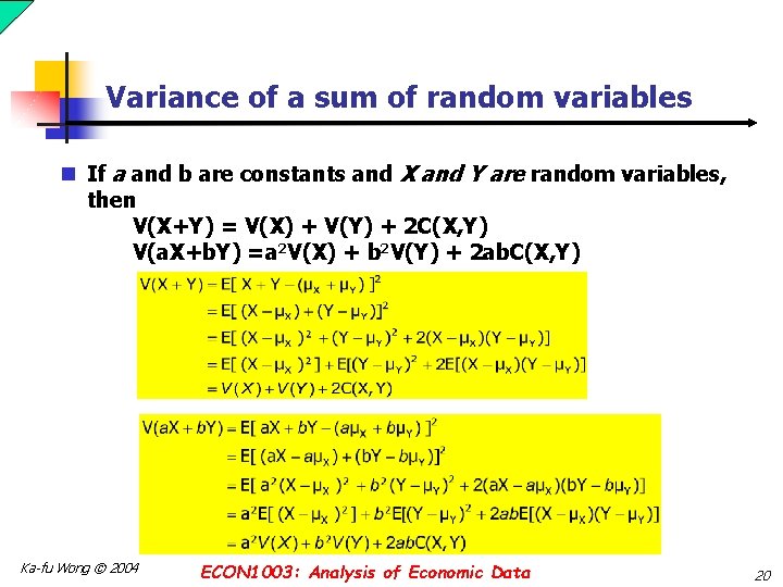
Variance of a sum of random variables n If a and b are constants and X and Y are random variables, then V(X+Y) = V(X) + V(Y) + 2 C(X, Y) V(a. X+b. Y) =a 2 V(X) + b 2 V(Y) + 2 ab. C(X, Y) Ka-fu Wong © 2004 ECON 1003: Analysis of Economic Data 20

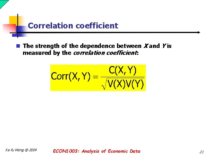
Correlation coefficient n The strength of the dependence between X and Y is measured

Importance of Normal Distribution 1. Describes many random processes or continuous phenomena 2. Basis

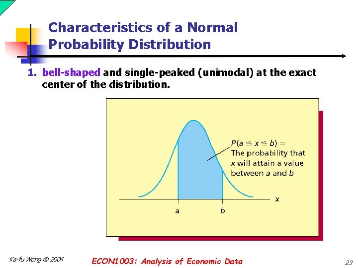
Characteristics of a Normal Probability Distribution 1. bell-shaped and single-peaked (unimodal) at the exact

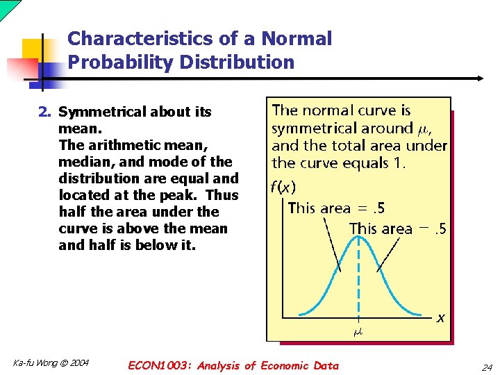
Characteristics of a Normal Probability Distribution 2. Symmetrical about its mean. The arithmetic mean, median, and mode of the distribution are equal and located at the peak. Thus half the area under the curve is above the mean and half is below it. Ka-fu Wong © 2004 ECON 1003: Analysis of Economic Data 24

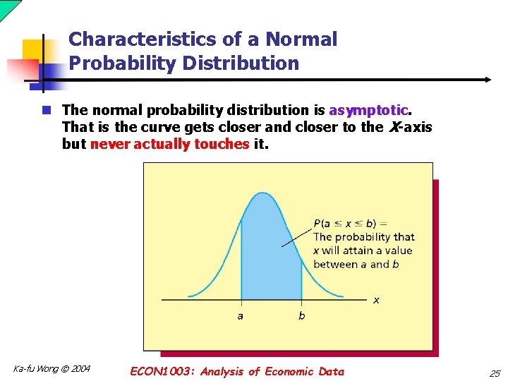
Characteristics of a Normal Probability Distribution n The normal probability distribution is asymptotic. That is the curve gets closer and closer to the X-axis but never actually touches it. Ka-fu Wong © 2004 ECON 1003: Analysis of Economic Data 25

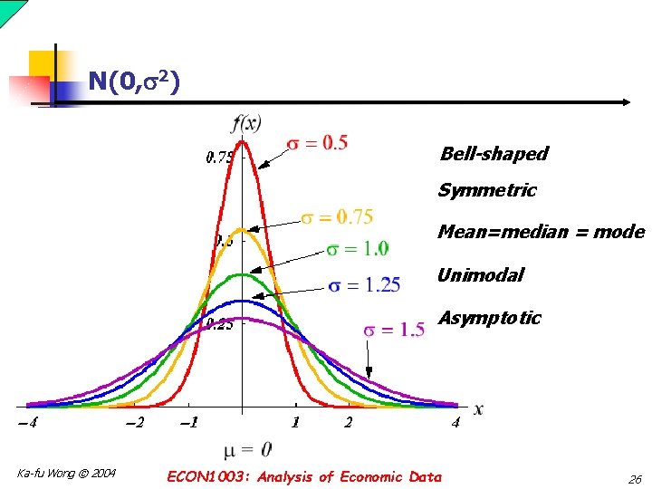
N(0, 2) Bell-shaped Symmetric Mean=median = mode Unimodal Asymptotic Ka-fu Wong © 2004 ECON

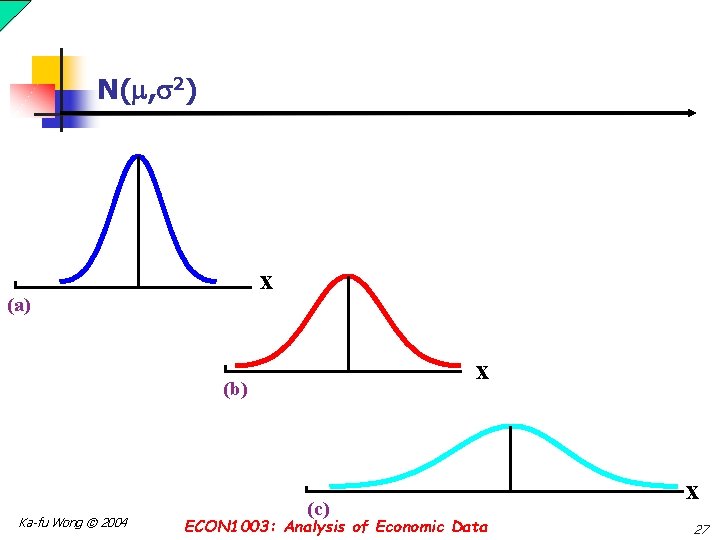
N( , 2) x (a) x (b) Ka-fu Wong © 2004 (c) ECON 1003:

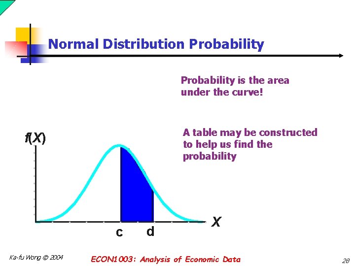
Normal Distribution Probability is the area under the curve! A table may be constructed

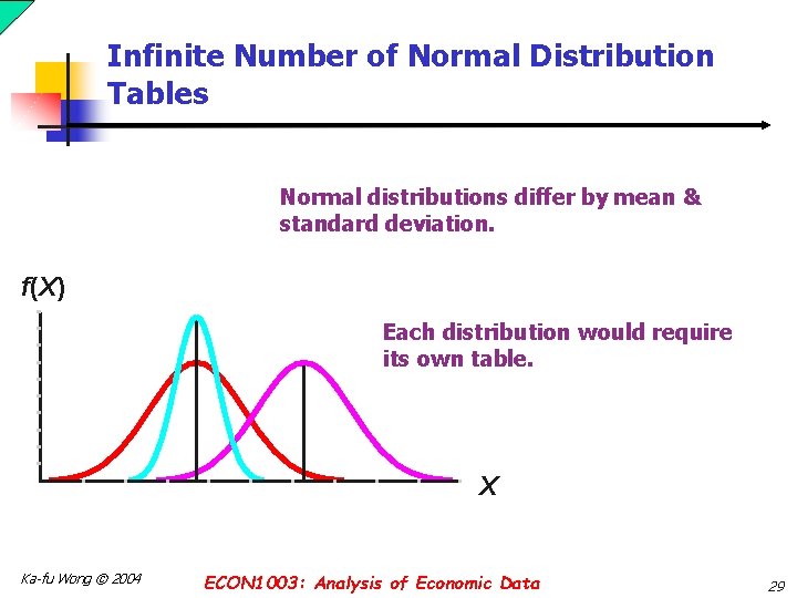
Infinite Number of Normal Distribution Tables Normal distributions differ by mean & standard deviation. f(X) Each distribution would require its own table. X Ka-fu Wong © 2004 ECON 1003: Analysis of Economic Data 29

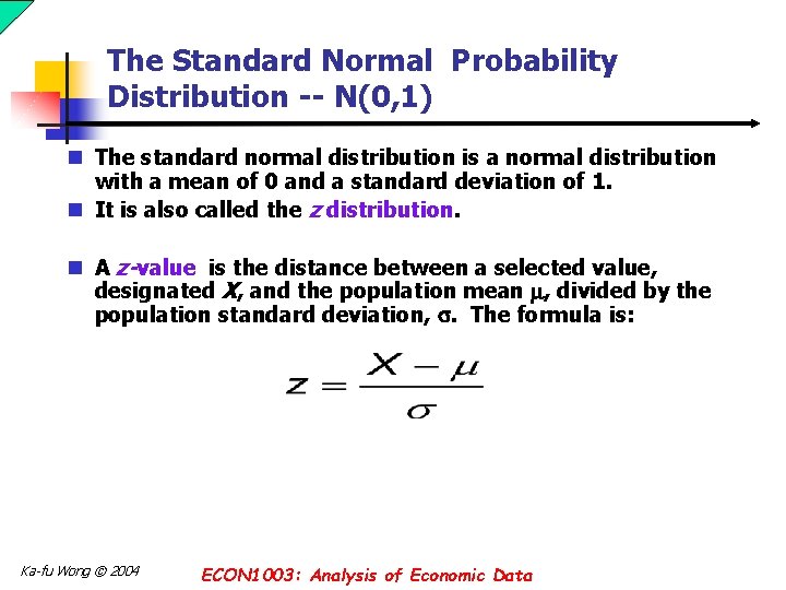
The Standard Normal Probability Distribution -- N(0, 1) n The standard normal distribution is a normal distribution with a mean of 0 and a standard deviation of 1. n It is also called the z distribution. n A z-value is the distance between a selected value, designated X, and the population mean , divided by the population standard deviation, . The formula is: Ka-fu Wong © 2004 ECON 1003: Analysis of Economic Data

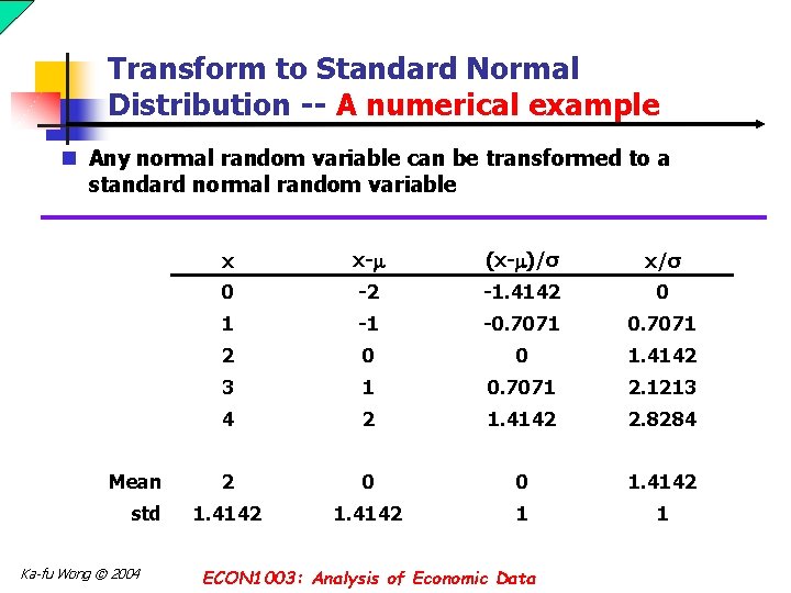
Transform to Standard Normal Distribution -- A numerical example n Any normal random variable can be transformed to a standard normal random variable Mean std Ka-fu Wong © 2004 x x- (x- )/σ x/σ 0 -2 -1. 4142 0 1 -1 -0. 7071 2 0 0 1. 4142 3 1 0. 7071 2. 1213 4 2 1. 4142 2. 8284 2 0 0 1. 4142 1 1 ECON 1003: Analysis of Economic Data

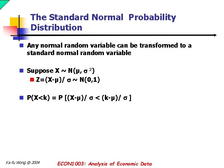
The Standard Normal Probability Distribution n Any normal random variable can be transformed to a standard normal random variable n Suppose X ~ N(µ, 2) n Z=(X-µ)/ ~ N(0, 1) n P(X<k) = P [(X-µ)/ < (k-µ)/ ] Ka-fu Wong © 2004 ECON 1003: Analysis of Economic Data

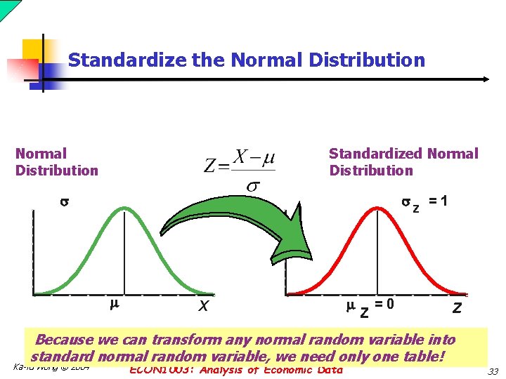
Standardize the Normal Distribution Standardized Normal Distribution z = 1 X Z =0 Z Because we can transform any normal random variable into standard normal random variable, we need only one table! Ka-fu Wong © 2004 ECON 1003: Analysis of Economic Data 33

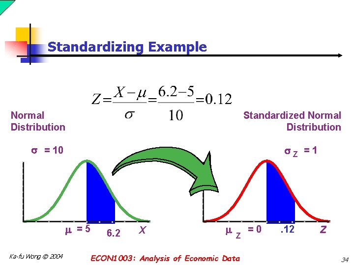
Standardizing Example Normal Distribution Standardized Normal Distribution = 10 Z =1 =5 Ka-fu Wong

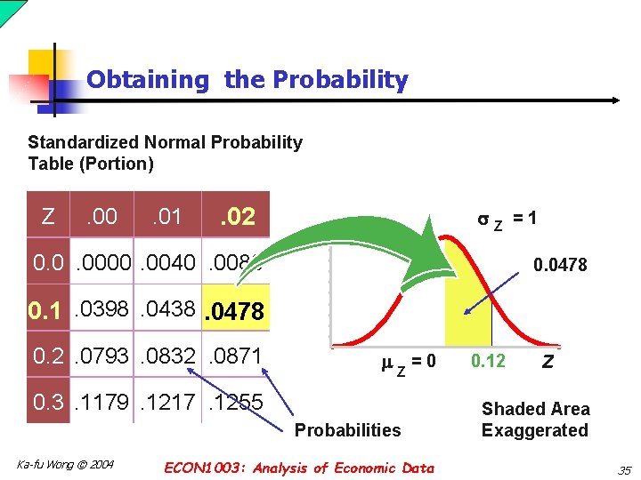
Obtaining the Probability Standardized Normal Probability Table (Portion) Z . 00 . 01 . 02 Z 0. 0. 0000. 0040. 0080 =1 0. 0478 0. 1. 0398. 0438. 0478 0. 2. 0793. 0832. 0871 Z =0 0. 3. 1179. 1217. 1255 Probabilities Ka-fu Wong © 2004 ECON 1003: Analysis of Economic Data 0. 12 Z Shaded Area Exaggerated 35

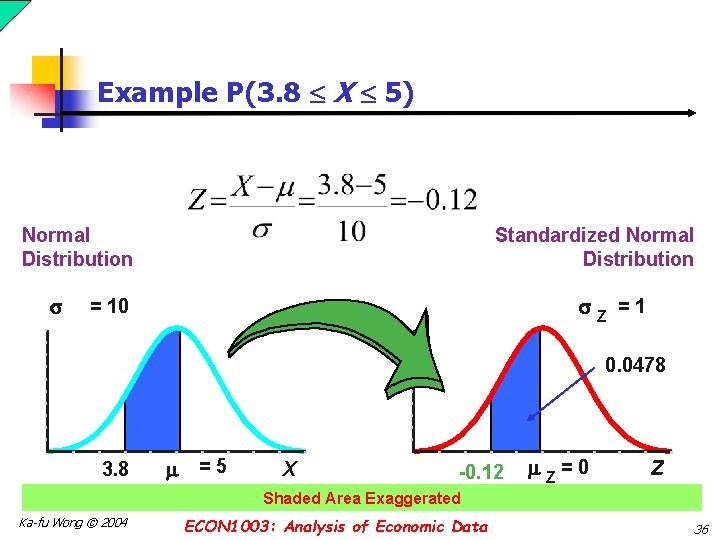
Example P(3. 8 X 5) Normal Distribution Standardized Normal Distribution = 10 Z =1

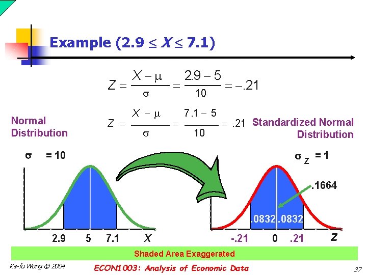
Example (2. 9 X 7. 1) Z Normal Distribution Z X X 2. 9 5 10 7. 1 5 10 . 21 Standardized Normal Distribution = 10 Z =1. 1664 . 0832 2. 9 5 7. 1 X -. 21 0 . 21 Z Shaded Area Exaggerated Ka-fu Wong © 2004 ECON 1003: Analysis of Economic Data 37

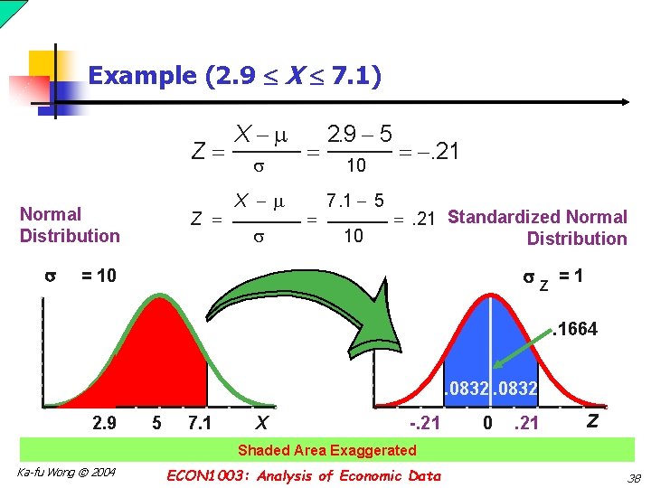
Example (2. 9 X 7. 1) Z Normal Distribution Z X X 2. 9 5 10 7. 1 5 10 . 21 Standardized Normal Distribution = 10 Z =1. 1664 . 0832 2. 9 5 7. 1 X -. 21 0 . 21 Z Shaded Area Exaggerated Ka-fu Wong © 2004 ECON 1003: Analysis of Economic Data 38

Example P(X 8) Normal Distribution Z X 8 5 10 . 30 Standardized Normal Distribution = 10 Z . 5000 =1 . 3821 . 1179 =5 8 X Z=0 . 30 Z Shaded Area Exaggerated Ka-fu Wong © 2004 ECON 1003: Analysis of Economic Data 39

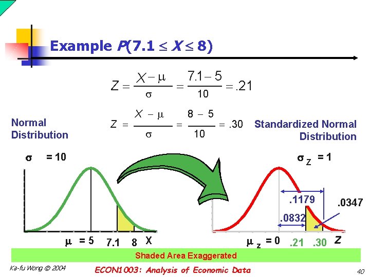
Example P(7. 1 X 8) Z Normal Distribution Z X X 7. 1 5 10 8 5 10 . 21 . 30 Standardized Normal Distribution Z =1 = 10 . 1179 . 0347 . 0832 =5 7. 1 8 X z = 0. 21. 30 Z Shaded Area Exaggerated Ka-fu Wong © 2004 ECON 1003: Analysis of Economic Data 40

Normal Distribution Thinking Challenge n You work in Quality Control for GE. Light bulb life has a normal distribution with µ= 2000 hours & = 200 hours. What’s the probability that a bulb will last n between 2000 & 2400 hours? n less than 1470 hours? Ka-fu Wong © 2004 ECON 1003: Analysis of Economic Data 41

Solution P(2000 X 2400) P(2000<X<2400) = P [(2000 -µ)/ <(X-µ)/ < (2400 -µ)/ ] = P[(X-µ)/ < (2400 -µ)/ ] – P [(X-µ)/ < (2000 -µ)/ ] = P[(X-µ)/ < (2400 -µ)/ ] – 0. 5 Normal X Distribution Z = 200 2400 2000 200 Standardized Normal Distribution 2. 0 Z = 1. 4772 = 2000 2400 X Shaded Area Exaggerated Ka-fu Wong © 2004 Z= 0 ECON 1003: Analysis of Economic Data 2. 0 Z 42

Solution P(X 1470) P(X<1470) = P [(X-µ)/ < (1470 -µ)/ ] Z Normal Distribution X 1470 2000 2. 65 Standardized Normal Distribution Z = 1 = 200 . 5000. 4960 . 0040 1470 = 2000 X -2. 65 Shaded Area Exaggerated Ka-fu Wong © 2004 ECON 1003: Analysis of Economic Data Z= 0 Z 43

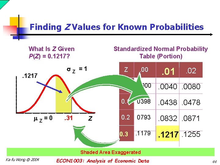
Finding Z Values for Known Probabilities What Is Z Given P(Z) = 0. 1217? . 1217 Z =0 Z . 31 Standardized Normal Probability Table (Portion) =1 Z . 00 0. 0 . 0000 . 0040. 0080 0. 1. 0398 . 0438. 0478 0. 2. 0793 . 0832. 0871 . 1179 . 1217. 1255 0. 3 . 02 Shaded Area Exaggerated Ka-fu Wong © 2004 ECON 1003: Analysis of Economic Data 44

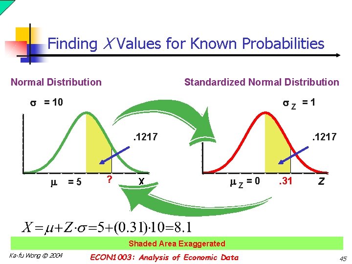
Finding X Values for Known Probabilities Normal Distribution Standardized Normal Distribution = 10 Z =1. 1217 =5 ? X . 1217 Z =0 . 31 Z Shaded Area Exaggerated Ka-fu Wong © 2004 ECON 1003: Analysis of Economic Data 45

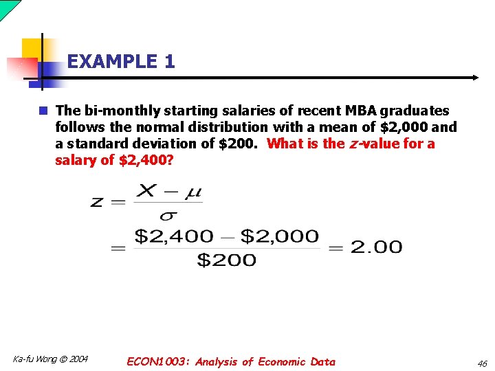
EXAMPLE 1 n The bi-monthly starting salaries of recent MBA graduates follows the normal distribution with a mean of $2, 000 and a standard deviation of $200. What is the z-value for a salary of $2, 400? Ka-fu Wong © 2004 ECON 1003: Analysis of Economic Data 46

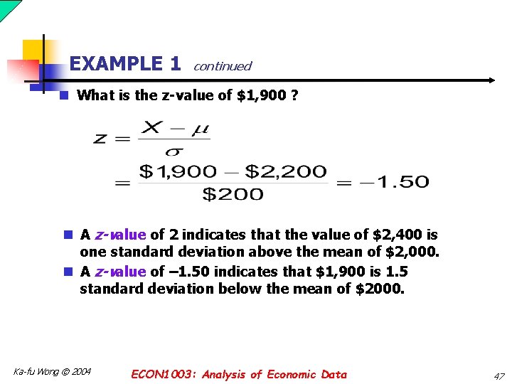
EXAMPLE 1 continued n What is the z-value of $1, 900 ? n A z-value of 2 indicates that the value of $2, 400 is one standard deviation above the mean of $2, 000. n A z-value of – 1. 50 indicates that $1, 900 is 1. 5 standard deviation below the mean of $2000. Ka-fu Wong © 2004 ECON 1003: Analysis of Economic Data 47

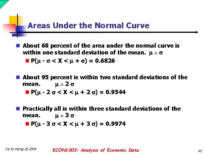
Areas Under the Normal Curve n About 68 percent of the area under the normal curve is within one standard deviation of the mean. ± n P( - < X < + ) = 0. 6826 n About 95 percent is within two standard deviations of the mean. ± 2 n P( - 2 < X < + 2 ) = 0. 9544 n Practically all is within three standard deviations of the mean. ± 3 n P( - 3 < X < + 3 ) = 0. 9974 Ka-fu Wong © 2004 ECON 1003: Analysis of Economic Data 48

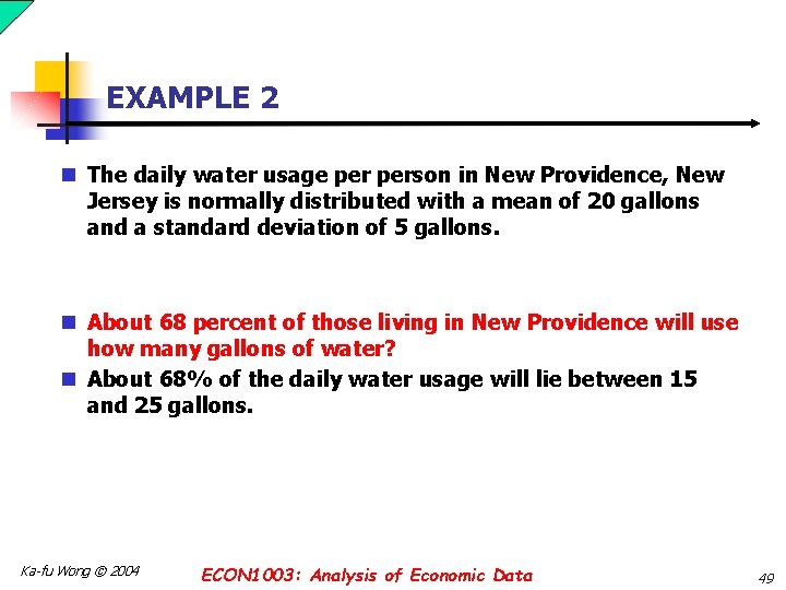
EXAMPLE 2 n The daily water usage person in New Providence, New Jersey is normally distributed with a mean of 20 gallons and a standard deviation of 5 gallons. n About 68 percent of those living in New Providence will use how many gallons of water? n About 68% of the daily water usage will lie between 15 and 25 gallons. Ka-fu Wong © 2004 ECON 1003: Analysis of Economic Data 49

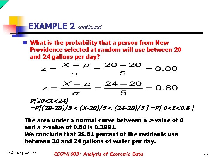
EXAMPLE 2 continued n What is the probability that a person from New Providence selected at random will use between 20 and 24 gallons per day? P(20<X<24) =P[(20 -20)/5 < (X-20)/5 < (24 -20)/5 ] =P[ 0<Z<0. 8 ] The area under a normal curve between a z-value of 0 and a z-value of 0. 80 is 0. 2881. We conclude that 28. 81 percent of the residents use between 20 and 24 gallons of water per day. Ka-fu Wong © 2004 ECON 1003: Analysis of Economic Data 50

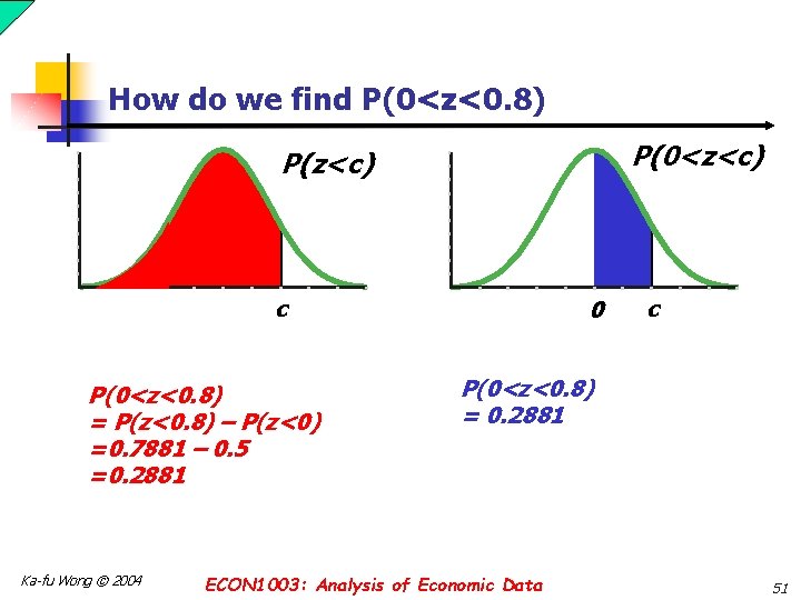
How do we find P(0<z<0. 8) P(0<z<c) P(z<c) c P(0<z<0. 8) = P(z<0. 8)

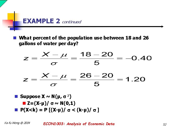
EXAMPLE 2 continued n What percent of the population use between 18 and 26 gallons of water per day? n Suppose X ~ N(µ, 2) n Z=(X-µ)/ ~ N(0, 1) n P(X<k) = P [(X-µ)/ < (k-µ)/ ] Ka-fu Wong © 2004 ECON 1003: Analysis of Economic Data 52

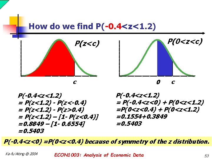
How do we find P(-0. 4<z<1. 2) P(0<z<c) P(z<c) c P(-0. 4<z<1. 2) = P(z<1. 2) - P(z<-0. 4) = P(z<1. 2) - P(z>0. 4) = P(z<1. 2) – [1 - P(z<0. 4)] =0. 8849 – [1 - 0. 6554] =0. 5403 0 c P(-0. 4<z<1. 2) = P(-0. 4<z<0) + P(0<z<1. 2) =P(0<z<0. 4) + P(0<z<1. 2) =0. 1554+0. 3849 =0. 5403 P(-0. 4<z<0) =P(0<z<0. 4) because of symmetry of the z distribution. Ka-fu Wong © 2004 ECON 1003: Analysis of Economic Data 53

EXAMPLE 3 n Professor Mann has determined that the scores in his statistics course are approximately normally distributed with a mean of 72 and a standard deviation of 5. He announces to the class that the top 15 percent of the scores will earn an A. n What is the lowest score a student can earn and still receive an A? Ka-fu Wong © 2004 ECON 1003: Analysis of Economic Data 54

Example 3 continued n To begin let k be the score that separates an A from a B. n 15 percent of the students score more than k, then 35 percent must score between the mean of 72 and k. n Write down the relation between k and the probability: n P(X>k) = 0. 15 and P(X<k) =1 -P(X>k) = 0. 85 n Transform X into z: n P[(X-72)/5) < (k-72)/5 ] = P[z < (k-72)/5] n P[0<z < s] =0. 85 -0. 5 = 0. 35 n Find s from table: n P[0<z<1. 04]=0. 35 n Compute k: n (k-72)/5=1. 04 implies K=77. 2 Those with a score of 77. 2 or more earn an A. Ka-fu Wong © 2004 ECON 1003: Analysis of Economic Data 55

The Normal Approximation to the Binomial n The normal distribution (a continuous distribution) yields a good approximation of the binomial distribution (a discrete distribution) for large values of n. n The normal probability distribution is generally a good approximation to the binomial probability distribution when n and n(1 - ) are both greater than 5. Why can we approximate binomial by normal? Because of the Central Limit Theorem. Ka-fu Wong © 2004 ECON 1003: Analysis of Economic Data 56

The Normal Approximation continued Recall for the binomial experiment: n There are only two mutually exclusive outcomes (success or failure) on each trial. n A binomial distribution results from counting the number of successes. n Each trial is independent. n The probability is fixed from trial to trial, and the number of trials n is also fixed. Ka-fu Wong © 2004 ECON 1003: Analysis of Economic Data 57

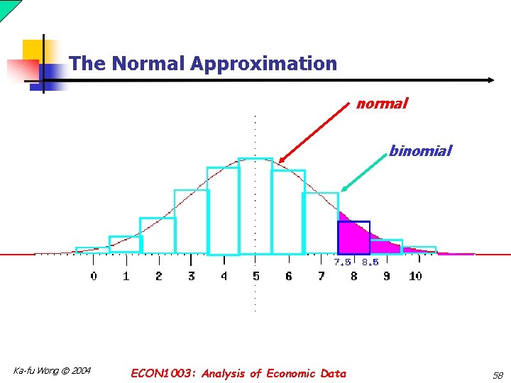
The Normal Approximation normal binomial Ka-fu Wong © 2004 ECON 1003: Analysis of Economic

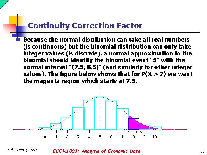
Continuity Correction Factor n Because the normal distribution can take all real numbers (is continuous) but the binomial distribution can only take integer values (is discrete), a normal approximation to the binomial should identify the binomial event "8" with the normal interval "(7. 5, 8. 5)" (and similarly for other integer values). The figure below shows that for P(X > 7) we want the magenta region which starts at 7. 5. Ka-fu Wong © 2004 ECON 1003: Analysis of Economic Data 59

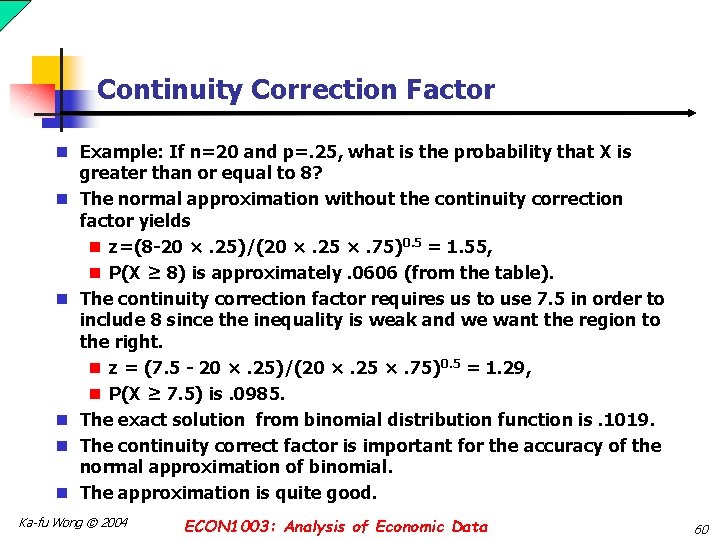
Continuity Correction Factor n Example: If n=20 and p=. 25, what is the probability that X is greater than or equal to 8? n The normal approximation without the continuity correction factor yields n z=(8 -20 ×. 25)/(20 ×. 25 ×. 75)0. 5 = 1. 55, n P(X ≥ 8) is approximately. 0606 (from the table). n The continuity correction factor requires us to use 7. 5 in order to include 8 since the inequality is weak and we want the region to the right. n z = (7. 5 - 20 ×. 25)/(20 ×. 25 ×. 75)0. 5 = 1. 29, n P(X ≥ 7. 5) is. 0985. n The exact solution from binomial distribution function is. 1019. n The continuity correct factor is important for the accuracy of the normal approximation of binomial. n The approximation is quite good. Ka-fu Wong © 2004 ECON 1003: Analysis of Economic Data 60

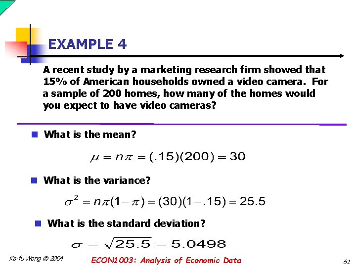
EXAMPLE 4 A recent study by a marketing research firm showed that 15% of American households owned a video camera. For a sample of 200 homes, how many of the homes would you expect to have video cameras? n What is the mean? n What is the variance? n What is the standard deviation? Ka-fu Wong © 2004 ECON 1003: Analysis of Economic Data 61

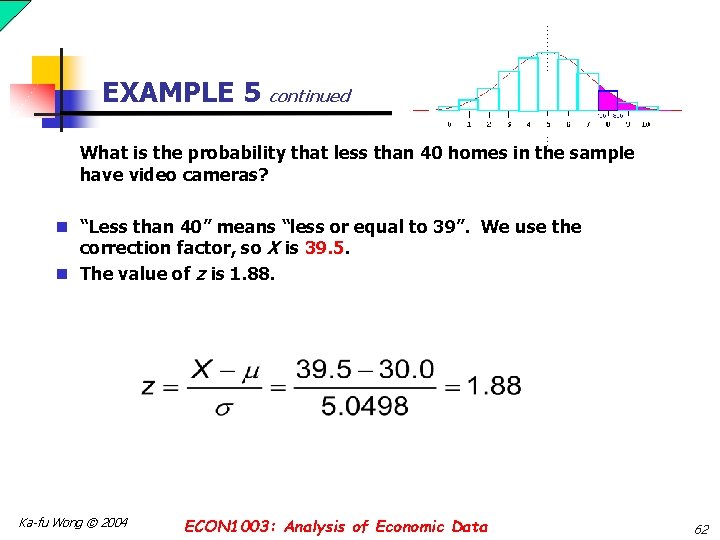
EXAMPLE 5 continued What is the probability that less than 40 homes in the sample have video cameras? n “Less than 40” means “less or equal to 39”. We use the correction factor, so X is 39. 5. n The value of z is 1. 88. Ka-fu Wong © 2004 ECON 1003: Analysis of Economic Data 62

Example 4 continued n From Standard Normal Table the area between 0 and 1. 88 on the z scale is. 4699. n So the area to the left of 1. 88 is. 5000 +. 4699 =. 9699. n The likelihood that less than 40 of the 200 homes have a video camera is about 97%. Ka-fu Wong © 2004 ECON 1003: Analysis of Economic Data 63