Lesson 4 Part B Forecasting Trend Projection Regression

Lesson 4 - Part B Forecasting • Trend Projection • Regression Analysis • Trend and Seasonal Components

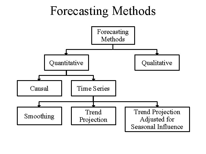
Forecasting Methods Quantitative Causal Time Series Smoothing Trend Projection Qualitative Trend Projection Adjusted for Seasonal Influence

Trend Projection • If a time series exhibits a linear trend, the method of least squares may be used to determine a trend line (projection) for future forecasts. • Least squares, also used in regression analysis, determines the unique trend line forecast which minimizes the mean square error between the trend line forecasts and the actual observed values for the time series. • The independent variable is the time period and the dependent variable is the actual observed value in the time series.

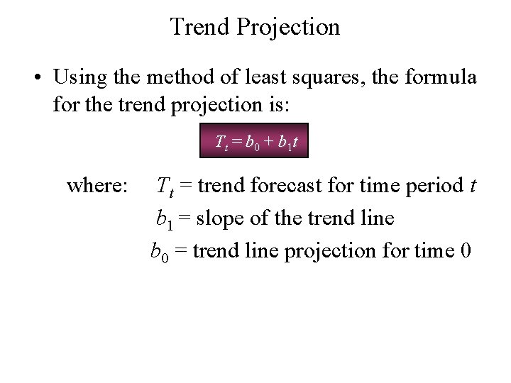
Trend Projection • Using the method of least squares, the formula for the trend projection is: Tt = b 0 + b 1 t where: Tt = trend forecast for time period t b 1 = slope of the trend line b 0 = trend line projection for time 0

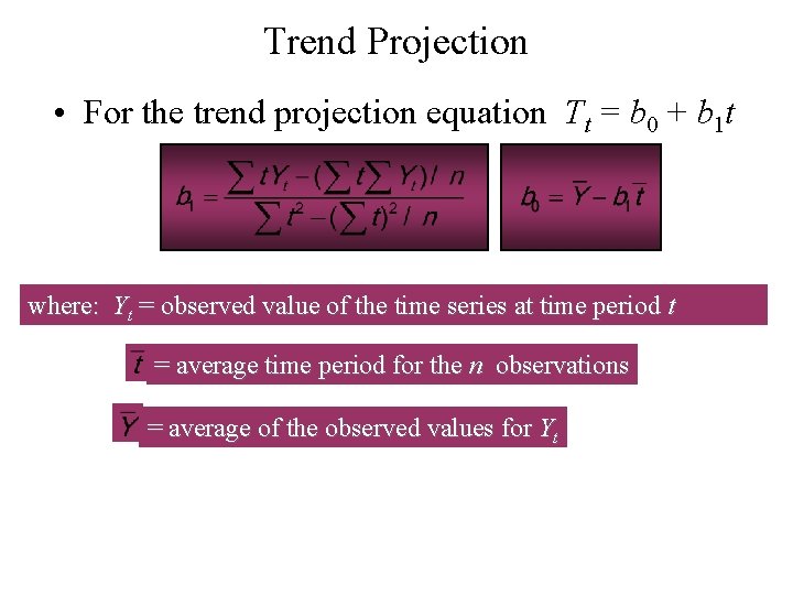
Trend Projection • For the trend projection equation Tt = b 0 + b 1 t where: Yt = observed value of the time series at time period t = average time period for the n observations = average of the observed values for Yt

Trend Projection • Example: Auger’s Plumbing Service The number of plumbing repair jobs performed by Auger's Plumbing Service in each of the last nine months is listed on the next slide. Forecast the number of repair jobs Auger's will perform in December using the least squares method.

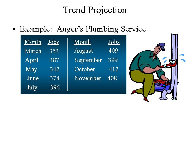
Trend Projection • Example: Auger’s Plumbing Service Month Jobs March 353 April 387 May 342 June 374 July 396 Month Jobs August 409 September 399 October 412 November 408

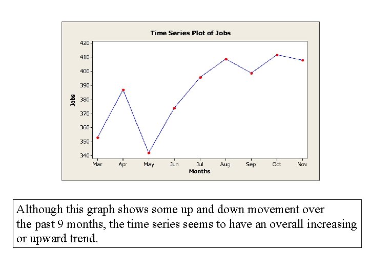
Although this graph shows some up and down movement over the past 9 months, the time series seems to have an overall increasing or upward trend.

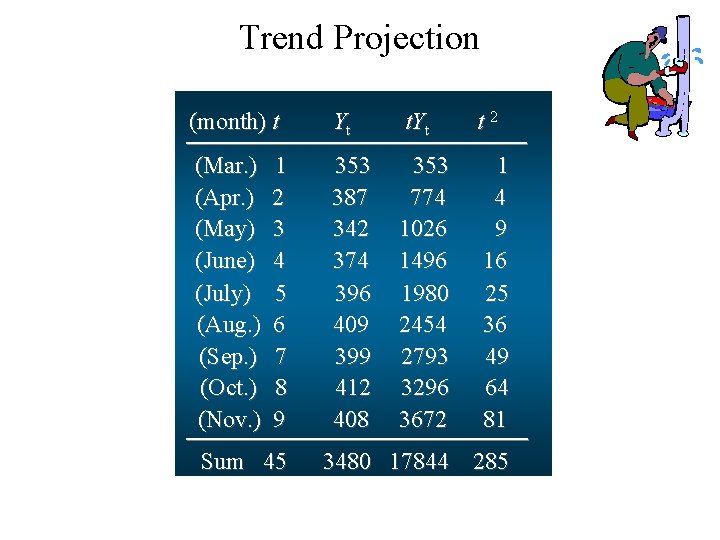
Trend Projection (month) t Yt t 2 (Mar. ) (Apr. ) (May) (June) (July) (Aug. ) (Sep. ) (Oct. ) (Nov. ) 353 387 342 374 396 409 399 412 408 353 774 1026 1496 1980 2454 2793 3296 3672 1 4 9 16 25 36 49 64 81 1 2 3 4 5 6 7 8 9 Sum 45 3480 17844 285

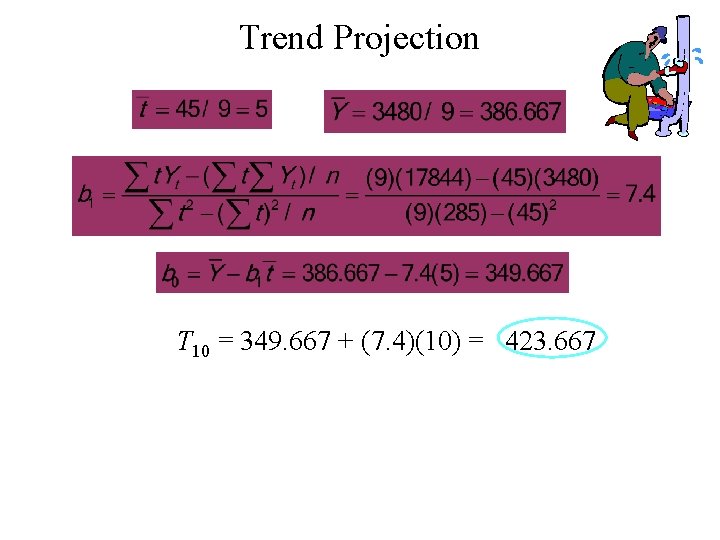
Trend Projection T 10 = 349. 667 + (7. 4)(10) = 423. 667

Trend Projection • Example: Auger’s Plumbing Service Forecast for December (Month 10) using a three-period (n = 3) weighted moving average with weights of. 6, . 3, and. 1 for the newest to oldest data, respectively. Then, compare this Month 10 weighted moving average forecast with the Month 10 trend projection forecast.

Trend Projection • Three-Month Weighted Moving Average The forecast for December will be the weighted average of the preceding three months: September, October, and November. F 10 =. 1 YSep. +. 3 YOct. +. 6 YNov. =. 1(399) +. 3(412) +. 6(408) = 408. 3 • Trend Projection F 10 = 423. 7 (from earlier slide)

Trend Projection • Conclusion Due to the positive trend component in the time series, the trend projection produced a forecast that is more in tune with the trend that exists. The weighted moving average, even with heavy (. 6) weight placed on the current period, produced a forecast that is lagging behind the changing data.

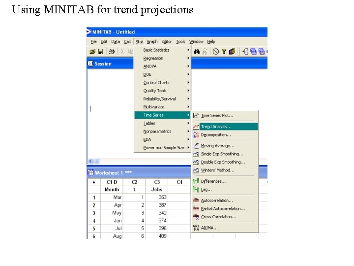
Using MINITAB for trend projections

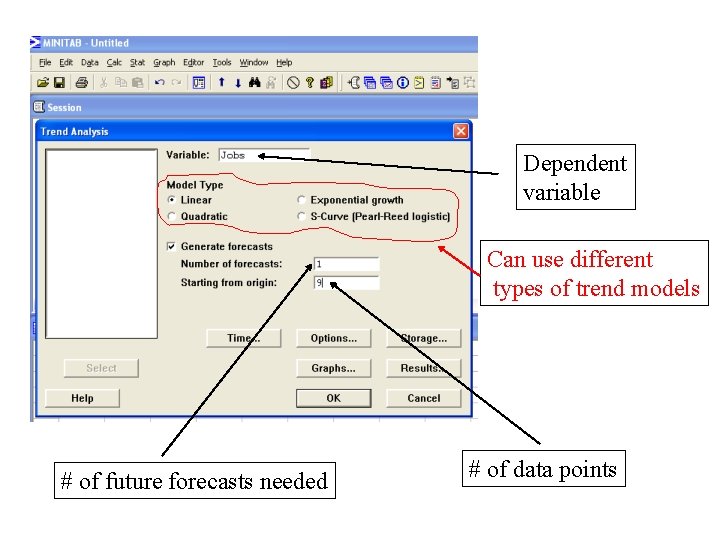
Dependent variable Can use different types of trend models # of future forecasts needed # of data points

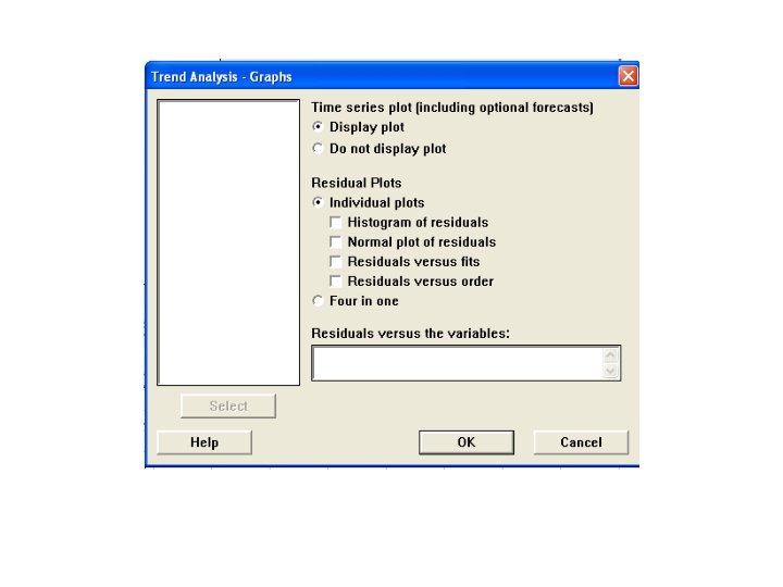
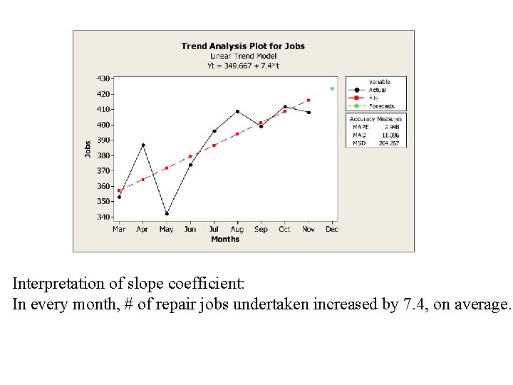
Interpretation of slope coefficient: In every month, # of repair jobs undertaken increased by 7. 4, on average.

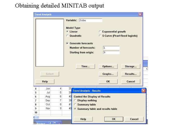
Obtaining detailed MINITAB output

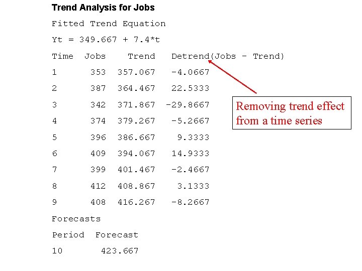
Trend Analysis for Jobs Fitted Trend Equation Yt = 349. 667 + 7. 4*t Time Jobs Trend 1 353 357. 067 -4. 0667 2 387 364. 467 22. 5333 3 342 371. 867 -29. 8667 4 379. 267 -5. 2667 5 396 386. 667 9. 3333 6 409 394. 067 14. 9333 7 399 401. 467 -2. 4667 8 412 408. 867 3. 1333 9 408 416. 267 -8. 2667 Forecasts Period 10 Forecast 423. 667 Detrend(Jobs – Trend) Removing trend effect from a time series

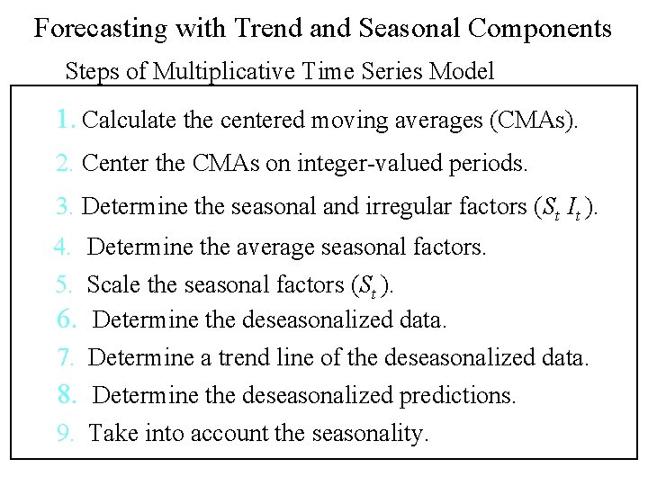
Forecasting with Trend and Seasonal Components Steps of Multiplicative Time Series Model 1. Calculate the centered moving averages (CMAs). 2. Center the CMAs on integer-valued periods. 3. Determine the seasonal and irregular factors (St It ). 4. Determine the average seasonal factors. 5. Scale the seasonal factors (St ). 6. Determine the deseasonalized data. 7. Determine a trend line of the deseasonalized data. 8. Determine the deseasonalized predictions. 9. Take into account the seasonality.

Forecasting with Trend and Seasonal Components • Example: Terry’s Tie Shop Business at Terry's Tie Shop can be viewed as falling into three distinct seasons: (1) Christmas (November and December); (2) Father's Day (late May to mid June); and (3) all other times. Average weekly sales ($) during each of the three seasons during the past four years are shown on the next slide.

Forecasting with Trend and Seasonal Components • Example: Terry’s Tie Shop Year 1 2 3 4 Season 1 2 1856 2012 1995 2168 2241 2306 2280 2408 3 985 1072 1105 1120 Determine a forecast for the average weekly sales in year 5 for each of the three seasons.

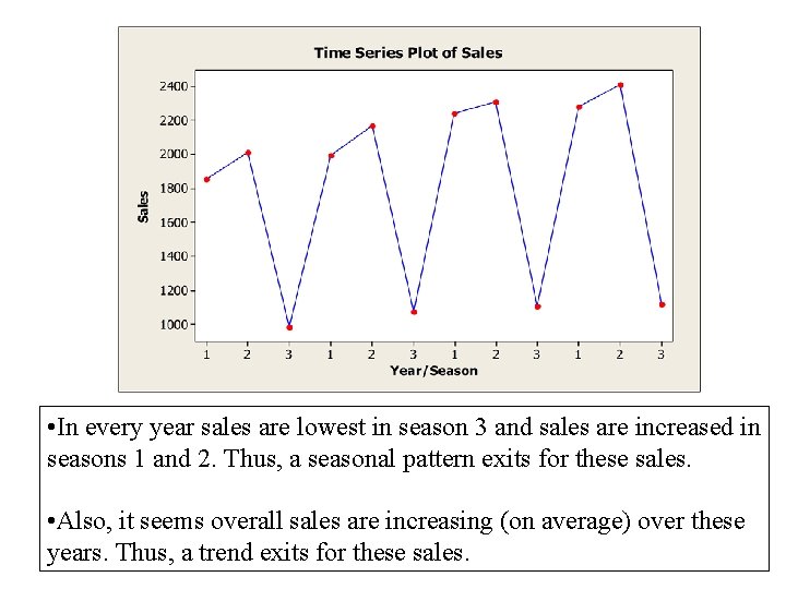
• In every year sales are lowest in season 3 and sales are increased in seasons 1 and 2. Thus, a seasonal pattern exits for these sales. • Also, it seems overall sales are increasing (on average) over these years. Thus, a trend exits for these sales.

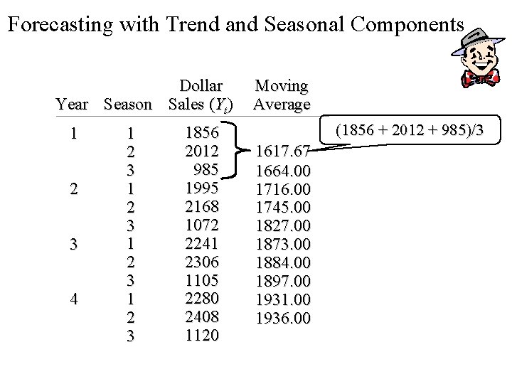
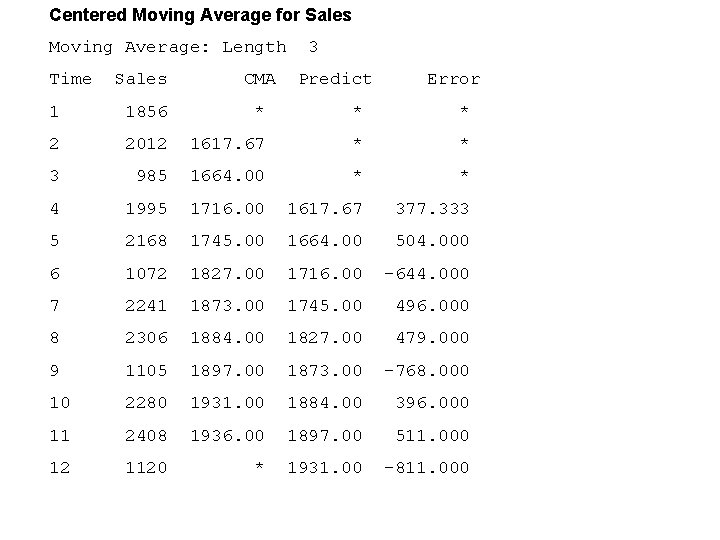
Forecasting with Trend and Seasonal Components Step 1. Calculate the centered moving averages. There are three distinct seasons in each year. Hence, take a three-season moving average to eliminate seasonal and irregular factors. For example: 1 st CMA = (1856 + 2012 + 985)/3 = 1617. 67 2 nd CMA = (2012 + 985 + 1995)/3 = 1664. 00 Etc.

Forecasting with Trend and Seasonal Components Step 2. Center the CMAs on integer-valued periods. The first centered moving average computed in step 1 (1617. 67) will be centered on season 2 of year 1. Note that the moving averages from step 1 center themselves on integer-valued periods because n is an odd number. If n is even, we have to compute the average of consecutive moving averages to get centered moving averages.

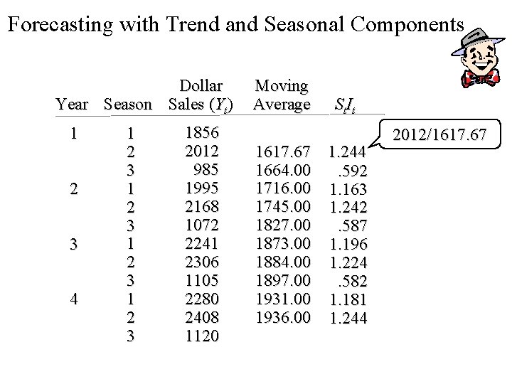
Forecasting with Trend and Seasonal Components Dollar Year Season Sales (Yt) 1 2 3 4 1 2 3 1856 2012 985 1995 2168 1072 2241 2306 1105 2280 2408 1120 Moving Average (1856 + 2012 + 985)/3 1617. 67 1664. 00 1716. 00 1745. 00 1827. 00 1873. 00 1884. 00 1897. 00 1931. 00 1936. 00

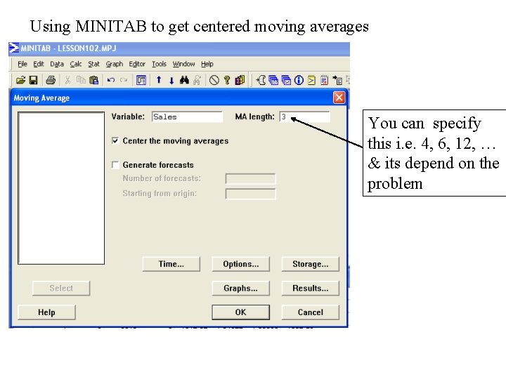
Using MINITAB to get centered moving averages You can specify this i. e. 4, 6, 12, … & its depend on the problem

Centered Moving Average for Sales Moving Average: Length Time 3 Sales CMA Predict Error 1 1856 * * * 2 2012 1617. 67 * * 3 985 1664. 00 * * 4 1995 1716. 00 1617. 67 377. 333 5 2168 1745. 00 1664. 00 504. 000 6 1072 1827. 00 1716. 00 -644. 000 7 2241 1873. 00 1745. 00 496. 000 8 2306 1884. 00 1827. 00 479. 000 9 1105 1897. 00 1873. 00 -768. 000 10 2280 1931. 00 1884. 00 396. 000 11 2408 1936. 00 1897. 00 511. 000 12 1120 * 1931. 00 -811. 000

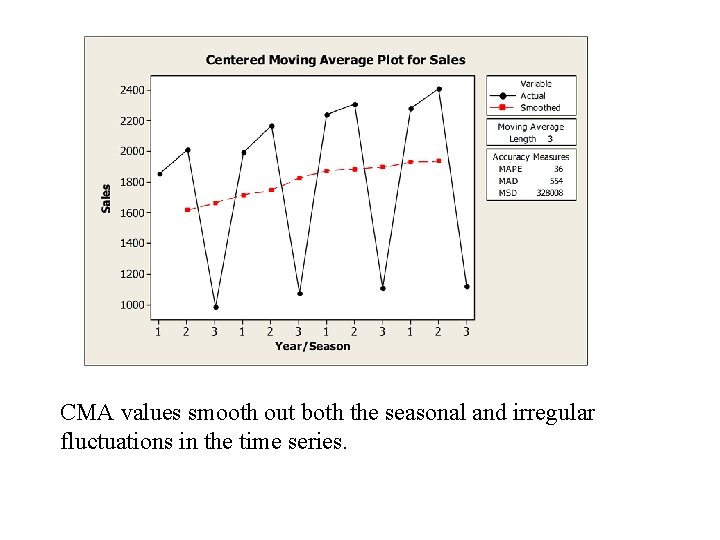
CMA values smooth out both the seasonal and irregular fluctuations in the time series.

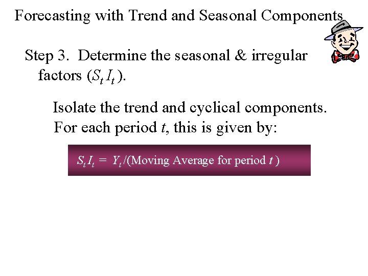
Forecasting with Trend and Seasonal Components Step 3. Determine the seasonal & irregular factors (St It ). Isolate the trend and cyclical components. For each period t, this is given by: St It = Yt /(Moving Average for period t )

Forecasting with Trend and Seasonal Components Dollar Year Season Sales (Yt) 1 2 3 4 1 2 3 1856 2012 985 1995 2168 1072 2241 2306 1105 2280 2408 1120 Moving Average St. It 1617. 67 1. 244 1664. 00. 592 1716. 00 1. 163 1745. 00 1. 242 1827. 00. 587 1873. 00 1. 196 1884. 00 1. 224 1897. 00. 582 1931. 00 1. 181 1936. 00 1. 244 2012/1617. 67

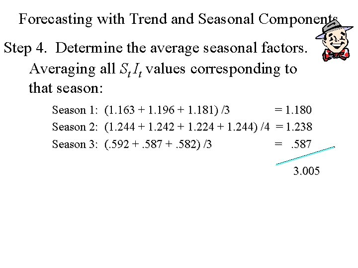
Forecasting with Trend and Seasonal Components Step 4. Determine the average seasonal factors. Averaging all St It values corresponding to that season: Season 1: Season 2: Season 3: (1. 163 + 1. 196 + 1. 181) /3 (1. 244 + 1. 242 + 1. 224 + 1. 244) /4 (. 592 +. 587 +. 582) /3 = 1. 180 = 1. 238 =. 587 3. 005

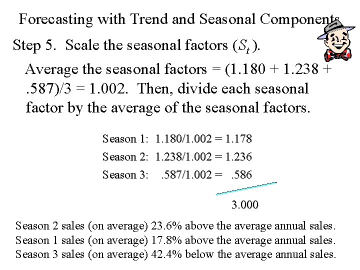
Forecasting with Trend and Seasonal Components Step 5. Scale the seasonal factors (St ). Average the seasonal factors = (1. 180 + 1. 238 +. 587)/3 = 1. 002. Then, divide each seasonal factor by the average of the seasonal factors. Season 1: 1. 180/1. 002 = 1. 178 Season 2: 1. 238/1. 002 = 1. 236 Season 3: . 587/1. 002 =. 586 3. 000 Season 2 sales (on average) 23. 6% above the average annual sales. Season 1 sales (on average) 17. 8% above the average annual sales. Season 3 sales (on average) 42. 4% below the average annual sales.

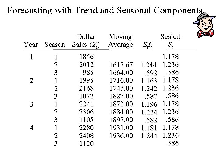
Forecasting with Trend and Seasonal Components Dollar Year Season Sales (Yt) 1 2 3 4 1 2 3 1856 2012 985 1995 2168 1072 2241 2306 1105 2280 2408 1120 Moving Average St. It 1617. 67 1. 244 1664. 00. 592 1716. 00 1. 163 1745. 00 1. 242 1827. 00. 587 1873. 00 1. 196 1884. 00 1. 224 1897. 00. 582 1931. 00 1. 181 1936. 00 1. 244 Scaled St 1. 178 1. 236. 586

Forecasting with Trend and Seasonal Components Step 6. Determine the deseasonalized data. Divide the data point values, Yt , by St.

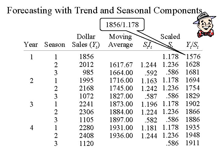
Forecasting with Trend and Seasonal Components 1856/1. 178 Dollar Year Season Sales (Yt) 1 2 3 4 1 2 3 1856 2012 985 1995 2168 1072 2241 2306 1105 2280 2408 1120 Moving Average St. It 1617. 67 1. 244 1664. 00. 592 1716. 00 1. 163 1745. 00 1. 242 1827. 00. 587 1873. 00 1. 196 1884. 00 1. 224 1897. 00. 582 1931. 00 1. 181 1936. 00 1. 244 Scaled Yt/St St 1. 178 1. 236. 586 1576 1628 1681 1694 1754 1829 1902 1866 1886 1935 1948 1911

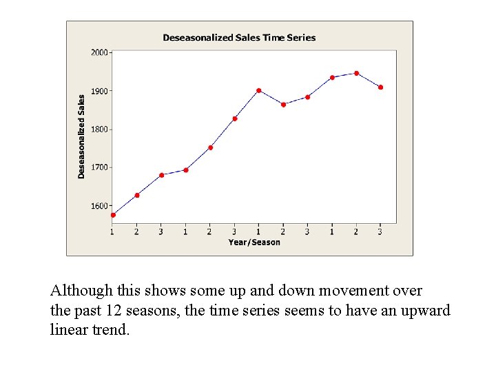
Although this shows some up and down movement over the past 12 seasons, the time series seems to have an upward linear trend.

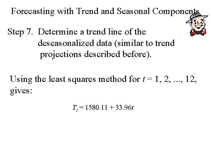
Forecasting with Trend and Seasonal Components Step 7. Determine a trend line of the deseasonalized data (similar to trend projections described before). Using the least squares method for t = 1, 2, . . . , 12, gives: Tt = 1580. 11 + 33. 96 t

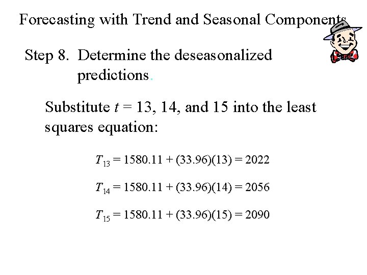
Forecasting with Trend and Seasonal Components Step 8. Determine the deseasonalized predictions. Substitute t = 13, 14, and 15 into the least squares equation: T 13 = 1580. 11 + (33. 96)(13) = 2022 T 14 = 1580. 11 + (33. 96)(14) = 2056 T 15 = 1580. 11 + (33. 96)(15) = 2090

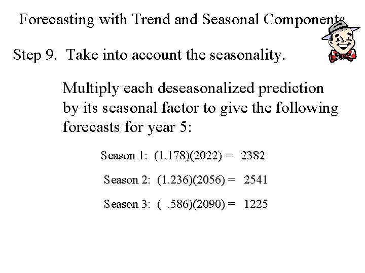
Forecasting with Trend and Seasonal Components Step 9. Take into account the seasonality. Multiply each deseasonalized prediction by its seasonal factor to give the following forecasts for year 5: Season 1: (1. 178)(2022) = 2382 Season 2: (1. 236)(2056) = 2541 Season 3: (. 586)(2090) = 1225

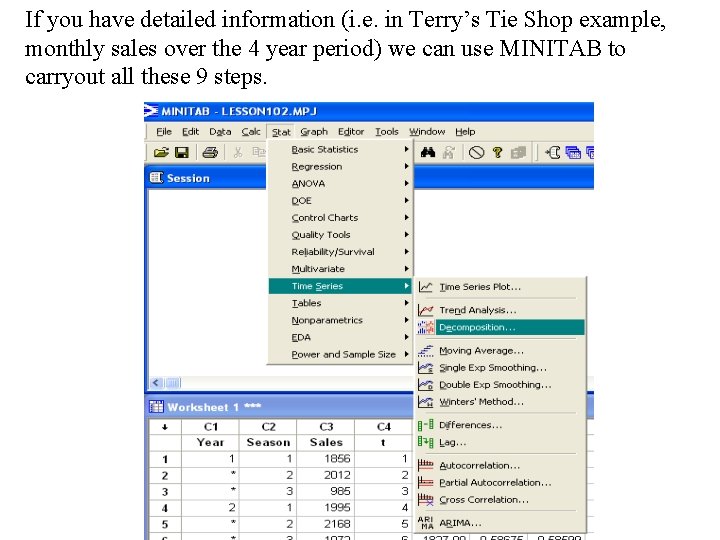
If you have detailed information (i. e. in Terry’s Tie Shop example, monthly sales over the 4 year period) we can use MINITAB to carryout all these 9 steps.

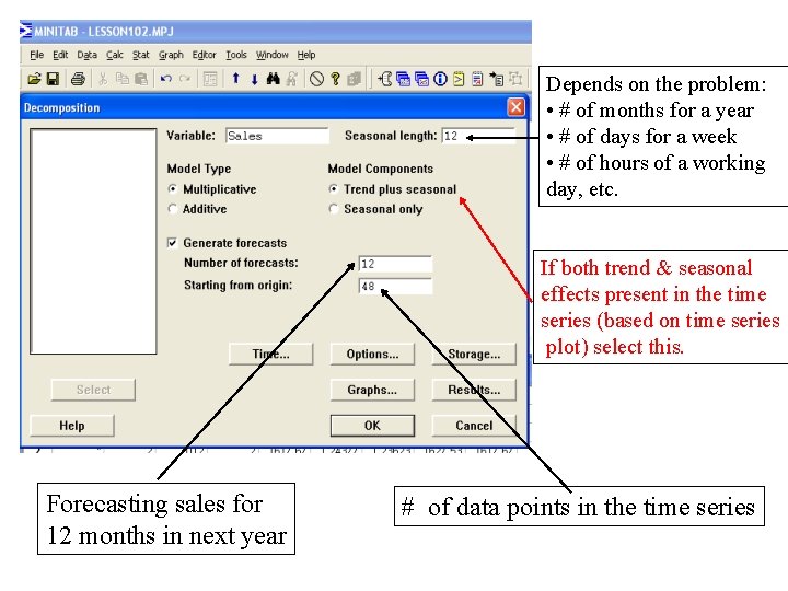
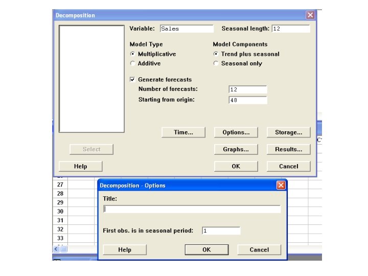
Depends on the problem: • # of months for a year • # of days for a week • # of hours of a working day, etc. If both trend & seasonal effects present in the time series (based on time series plot) select this. Forecasting sales for 12 months in next year # of data points in the time series