Lesson 4 Descriptive Procedures Procedures displaying associations between

Lesson 4 • Descriptive Procedures • Procedures displaying associations between 2 variables • Procedures FREQ, CORR, REG, SGPLOT • Comment and Option Statements • Program 4 in course notes • LSB: See syllabus • LSB: Chapter 11 – Debugging Programs

Program 4 DATA weight ; INFILE ‘C: SAS_Filestomhs. dat' ; INPUT @1 ptid $10. @12 clinic $1. @27 age 2. @30 sex 1. @58 height 4. @85 weight 5. @140 cholbl 3. ; bmi = (weight*703. 0768)/(height*height); RUN;

PROC FREQ DATA=weight; TABLES clinic sex ; TITLE 'Frequency Distribution of Clinical Center and Gender'; RUN; Frequency Distribution of Clinical Center and Gender The FREQ Procedure Cumulative clinic Frequency Percent ƒƒƒƒƒƒƒƒƒƒƒƒƒƒƒƒƒƒƒƒƒƒƒƒƒƒƒƒƒƒ A 18 18. 00 B 29 29. 00 47 47. 00 C 36 36. 00 83 83. 00 D 17 17. 00 100. 00 Cumulative sex Frequency Percent ƒƒƒƒƒƒƒƒƒƒƒƒƒƒƒƒƒƒƒƒƒƒƒƒƒƒƒƒ 1 73 73. 00 2 27 27. 00 100. 00

*2 -Way Frequency Tables ; PROC FREQ DATA=weight; TABLES sex*clinic ; TITLE 'Cross Tabulation of Clinical Center and Sex'; RUN; Row variable Column variable

Cross Tabulation of Clinical Center and Sex The FREQ Procedure Table of sex by clinic sex clinic Percent men in clinic A Frequency| Percent | Row Pct | Col Pct |A |B |C |D | Total -----+--------+--------+ 1 | 12 | 20 | 30 | 11 | 73 | 12. 00 | 20. 00 | 30. 00 | 11. 00 | 73. 00 | 16. 44 | 27. 40 | 41. 10 | 15. 07 | | 66. 67 | 68. 97 | 83. 33 | 64. 71 | -----+--------+--------+ 2 | 6 | 9 | 6 | 27 | 6. 00 | 9. 00 | 6. 00 | 27. 00 | 22. 22 | 33. 33 | 22. 22 | | 33. 33 | 31. 03 | 16. 67 | 35. 29 | -----+--------+--------+ Total 18 29 36 17 100 18. 00 29. 00 36. 00 17. 00 100. 00

* Getting only the counts ; PROC FREQ DATA=weight; TABLES sex*clinic / nopercent norow nocol; RUN; sex clinic Frequency|A |B |C |D Total -----+--------+--------+ 1 | 12 | 20 | 30 | 11 | 73 -----+--------+--------+ 2 | 6 | 9 | 6 | 27 -----+--------+--------+ Total 18 29 36 17 100

*Adding a two-way plot ; PROC FREQ DATA=weight; TABLES sex*clinic/ PLOTS=FREQPLOT(TWOWAY=GROUPHORIZONTAL); RUN;

OTHER USEFUL TABLE OPTIONS • CHISQ – performs chi-square analyses for 2 -way tables • MISSING – includes missing data as a separate category • LIST – makes condensed table (useful when looking at 3 -way or higher tables)

* Using PROC SGPLOT for bar charts; ODS GRAPHICS /WIDTH=300 px ; PROC SGPLOT; VBAR clinic; TITLE "Vertical Bar Chart of Clinical Center"; LABEL clinic = "Clinical Center"; Plot can be imbedded into an HTML document or kept as a separate file. The file can be inserted in Office documents.

* Same plot displayed horizontally; PROC SGPLOT; HBAR clinic; TITLE “Horizontal Bar Chart of Clinical Center"; LABEL clinic = "Clinical Center";

* DATALABEL puts values on top of bar; PROC SGPLOT; YAXIS LABEL = "Mean Cholesterol" VALUES = (0 to 300 by 50); VBAR clinic/RESPONSE=cholbl STAT=MEAN DATALABEL ; TITLE 'Mean Cholesterol by Clinical Center'; LABEL clinic = "Clinical Center"; RUN;

* LIMITSTAT adds SE bars; PROC SGPLOT NOAUTOLEGEND; YAXIS LABEL = "Mean Cholesterol" VALUES = (0 to 300 by 50); VBAR clinic/RESPONSE=cholbl STAT=MEAN LIMITSTAT=STDERR ; TITLE 'Mean Cholesterol by Clinical Center'; LABEL clinic = "Clinical Center"; RUN;

* Using SGPLOT to make regression plot; PROC SGPLOT DATA=weight; YAXIS LABEL = "Body Mass Index (BMI)" ; XAXIS LABEL = "Age (y)" ; REG X=age Y=bmi/CLM; WHERE sex = 2; TITLE 'Plot of BMI and Age for Women'; RUN;

* Using SGPANEL to make paneled graphs; proc format; value sex 1=‘Men’ 2=‘Women’; run; proc sgpanel noautolegend; panelby sex/novarname columns=2 spacing=5; rowaxis label = "BMI (kg/m 2)" ; colaxis label = "Age (y)" ; reg x=age y=bmi; format sex. ; TITLE 'Plot of BMI Verus Age for Men and Women'; RUN;

PROC CORR DATA=weight; VAR bmi age; WHERE gender = 2; TITLE 'Correlation of BMI and Age for Women'; RUN; Pearson Correlation Coefficients, N = 27 Prob > |r| under H 0: Rho=0 bmi age bmi 1. 00000 -0. 44397 0. 0203 age -0. 44397 0. 0203 1. 00000 Correlation Coefficient P-value testing if correlation is significantly different from zero

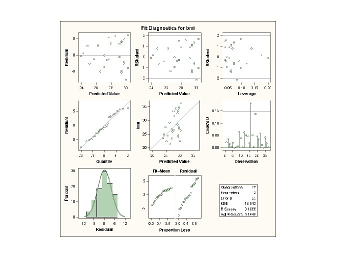
PROC REG DATA=weight ; MODEL bmi=age; WHERE gender = 2; TITLE 'Simple Linear Regression'; RUN; Partial Output Parameter Estimates Variable Intercept age DF Parameter Estimate Standard Error t Value Pr > |t| 1 1 43. 61312 -0. 28964 6. 40001 0. 11710 6. 81 -2. 47 <. 0001 0. 0205 Regression equation: bmi = 43. 61 - 0. 29*age *Note: many options for plotting within proc reg. ODS graphics on will produce many plots by default.

Fit plot from PROC REG

Using Comments in Program Two Purposes 1. Documenting your program 2. Temporarily delete part of a program See page 3 LSB

Examples of Comment Code * Run proc univariate for variable BMI; *-----------------------------------* High resolution graphs can also be produced. The following makes a plot of a histogram with the best fit normal curve and summary statistics. *-----------------------------------*; PROC MEANS DATA = weight N MEAN STDDEV; * CLASS sex ; VAR bmi; run; PROC MEANS DATA = weight /* N MEAN STDDEV*/; CLASS sex ; VAR bmi; run;

Temporarily Removing Code: Do not want to produce histogram but may want to run it at another time PROC UNIVARIATE DATA = weight; VAR bmi; /* HISTOGRAM bmi / NORMAL MIDPOINTS=20 to 40 by 2; INSET N MEAN STD MIN MAX = = = 'N' (5. 0) 'Mean' (5. 1) 'Sdev' (5. 1) 'Min' (5. 1) 'Max' (5. 1)/ POS=lm HEADER='Summary Statistics'; */ LABEL bmi = 'Body Mass Index (kg/m 2)'; RUN;

What is wrong with this program ? * This is my first SAS program DATA bp; INFILE. . . (more lines)

Option Statement OPTION NOCENTER LINESIZE = 78; OPTION NODATE NONUMBER; Many, many options (run PROC OPTIONS) Usually put at top of program Can put in autoexec. sas so they will always be in effect.

Debugging SAS Programs Finding and Correcting Errors Chapter 11: LSB

Checking the Log • It is always a good idea to check the log window. • Start at the beginning of the log file, and correct the first error. Sometimes one mistake can create many errors.

Missing Semicolons • Missing semicolons are the most common mistake to make. DATA weight INFILE ‘C: SAS_Filestomhs. dat' ; ERROR: No DATALINES or INFILE statement.

How to figure out what happened: • The Error said that there wasn’t a DATALINES or INFILE statement, but you know that there was one. • SAS must not have identified the INFILE statement as an INFILE statement. • Checking the code shows that SAS thought that the INFILE statement was part of the DATA statement because a semicolon was missing.

Another Missing Semicolon: PROC FREQ DATA=weight; TABLES sex clinic TITLE 'Frequency Distribution of Clinical Center and Gender'; RUN; ERROR: Variable TITLE not found.

How to figure out what happened: • SAS says that the variable TITLE wasn’t found. • You know that TITLE isn’t a variable. • SAS must think that TITLE is part of a list of variables. • There is no semicolon separating TITLE from the variables SEX and CLINIC!

Invalid Data • If SAS is expecting a number, but gets text instead, you can get invalid data notes. @ 12 clinic $1. • Is replaced with: @ 12 clinic 1. NOTE: Invalid data for clinic in line 1 12 -12

Mixing up PROCs PROC FREQ DATA=tdata; VAR clinic group educ ; 1016 VAR clinic group educ ; --180 ERROR 180 -322: Statement is not valid or it is used out of proper order.

Misspelled Variable in a PROC FREQ DATA=weight; TABLES sex clinic ; • Is replaced with: PROC FREQ DATA=weight; TABLES sex clinc ; • You get: ERROR: Variable CLINC not found.

Uninitialized Variables • From Program 4, if: bmi = (weight*703. 0768)/(height*height); • Is replaced with: bmi = (wieght*703. 0768)/(height*height); • You get: NOTE: Variable wieght is uninitialized.

What’s an Uninitialized Variable? • An uninitialized variable is a variable that SAS considers to be nonexistent. • This usually occurs when a variable name on the RHS of an equation is misspelled. • In the example, the error was caused by a misspelling—SAS had no variable called wieght.