Lesson 4 Arrays in MATLAB First round Lecturer

Lesson 4 Arrays in MATLAB First round Lecturer : Dr. Noam Amir Format Revised. 01 -17 -2007 r 3 CE 2002 -NTUST NOTE: (測試? !) – If marked, please try it by yourself. Seeing is believing. 建議 –This PPT is not always CORRECT. Please cut and paste the matlab code to prove it.

Outline: Testing arrays in MATLAB The colon operator Concatenating arrays in MATLAB Array indexing Array math Sorting and searching in arrays

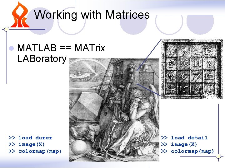
Working with Matrices l MATLAB == MATrix LABoratory >> load durer >> image(X) >> colormap(map) >> load detail >> image(X) >> colormap(map)

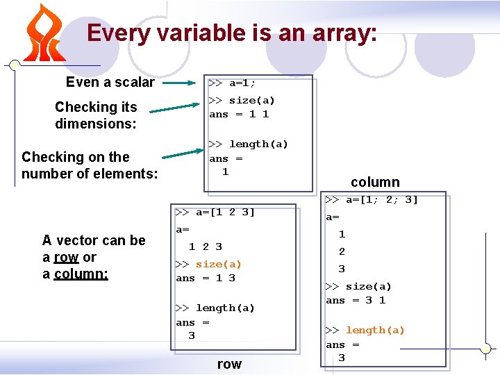
Every variable is an array: Even a scalar >> a=1; >> size(a) ans = 1 1 Checking its dimensions: >> length(a) ans = 1 Checking on the number of elements: >> a=[1 2 3] A vector can be a row or a column: a= 1 2 3 >> size(a) ans = 1 3 >> length(a) ans = 3 row column >> a=[1; 2; 3] a= 1 2 3 >> size(a) ans = 3 1 >> length(a) ans = 3

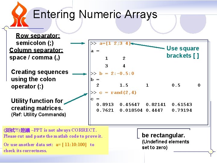
Entering Numeric Arrays Row separator: semicolon (; ) Column separator: space / comma (, ) Creating sequences using the colon operator (: ) Utility function for creating matrices. (Ref: Utility Commands) >> a=[1 2; 3 4] Use square brackets [ ] a = 1 2 3 4 >> b = 2: -0. 5: 0 b = 2 1. 5 1 >> c = rand(2, 4) c = 0. 8913 0. 45647 0. 82141 0. 7621 0. 018504 0. 4447 (測試? !)建議 –PPT is not always CORRECT. Please cut and paste the matlab code to prove it. Or use another data set: a= [ 11: 100] to check its correctness. 0. 5 0. 61543 0. 79194 Matrices must be rectangular. (Undefined elements set to zero) 0

Entering Numeric Arrays - cont. Using other MATLAB expressions Matrix element assignment >> w = [-2. 8, sqrt(-7), (3+5+6)*3/4] w = -2. 8 0 + 2. 6458 i 10. 5 >> x(3, 2) = 3. 5 x = 0 0 0 3. 5 >> w(2, 5) = 23 w = -2. 8 0 Any MATLAB expression can be entered as a matrix element 0 + 2. 6458 i 0 10. 5 0 0 23

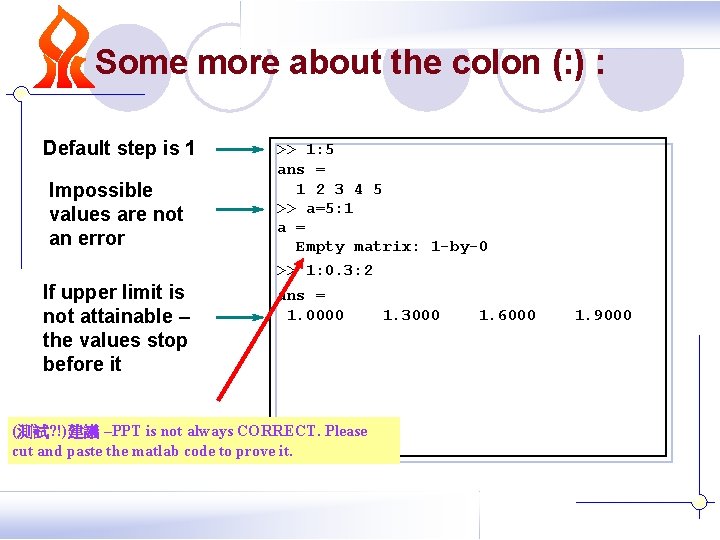
Some more about the colon (: ) : Default step is 1 Impossible values are not an error If upper limit is not attainable – the values stop before it >> 1: 5 ans = 1 2 3 4 5 >> a=5: 1 a = Empty matrix: 1 -by-0 >> 1: 0. 3: 2 ans = 1. 0000 (測試? !)建議 –PPT is not always CORRECT. Please cut and paste the matlab code to prove it. 1. 3000 1. 6000 1. 9000

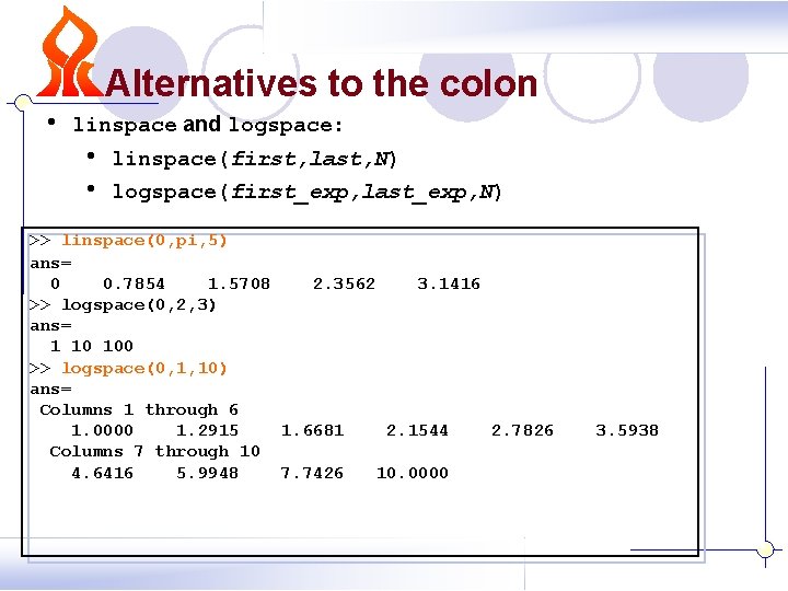
Alternatives to the colon • linspace and logspace: • • linspace(first, last, N) logspace(first_exp, last_exp, N) >> linspace(0, pi, 5) ans= 0 0. 7854 1. 5708 2. 3562 3. 1416 >> logspace(0, 2, 3) ans= 1 10 100 >> logspace(0, 1, 10) ans= Columns 1 through 6 1. 0000 1. 2915 1. 6681 2. 1544 2. 7826 Columns 7 through 10 4. 6416 5. 9948 7. 7426 10. 0000 3. 5938

Numerical Array Concatenation - [ ] Use [ ] to combine existing arrays as matrix “elements” Row separator: semicolon (; ) Column separator: space / comma (, ) Matrices must be rectangular. >> a=[1 2; 3 4] a = 1 2 3 4 Use square brackets [ ] >> cat_a=[a, 2*a; 3*a, 4*a; 5*a, 6*a] cat_a = 1 2 2 4 3 4 6 8 3 6 4 8 4*a 9 12 12 16 5 10 6 12 15 20 18 24 (測試? !)建議 –PPT is not always CORRECT. Please cut and paste the matlab code to prove it. Use another data set a = pascal(5) to see new result.

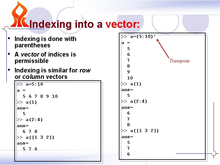
Indexing into a vector: • Indexing is done with parentheses • A vector of indices is permissible • Indexing is similar for row or column vectors >> a=5: 10 a = 5 6 7 8 9 10 >> a(1) ans= 5 >> a(2: 4) ans= 6 7 8 >> a([1 3 2]) ans= 5 7 6 >> a=(5: 10)’ a = 5 6 7 8 9 10 >> a(1) ans= 5 >> a(2: 4) ans= 6 7 8 >> a([1 3 2]) ans= 5 7 6 Transpose

Indexing into a matrix: A matrix has more than one dimension (維 度 ) - n So an index into a matrix has to address each dimension separately, e. g. : mat(3, 5) row ( 橫列 ) column (直行 ) BUT: n n n After all, a matrix is stored in memory as a string of elements And we can address that string of elements as a VECTOR! In other words – matrices in Matlab play magic functions. … let’s have a look:

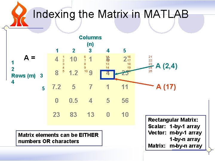
Indexing the Matrix in MATLAB Columns (n) 2 3 4 1 A= 1 2 Rows (m) 3 4 5 4 8 1 2 3 4 5 10 1. 2 6 7 8 9 10 1 9 11 12 13 14 15 5 16 6 217 4 25 18 19 20 7. 2 5 7 1 11 0 0. 5 4 5 56 23 83 13 0 10 Matrix elements can be EITHER numbers OR characters 21 22 23 24 25 A (2, 4) A (17) Rectangular Matrix: Scalar: 1 -by-1 array Vector: m-by-1 array 1 -by-n array Matrix: m-by-n array

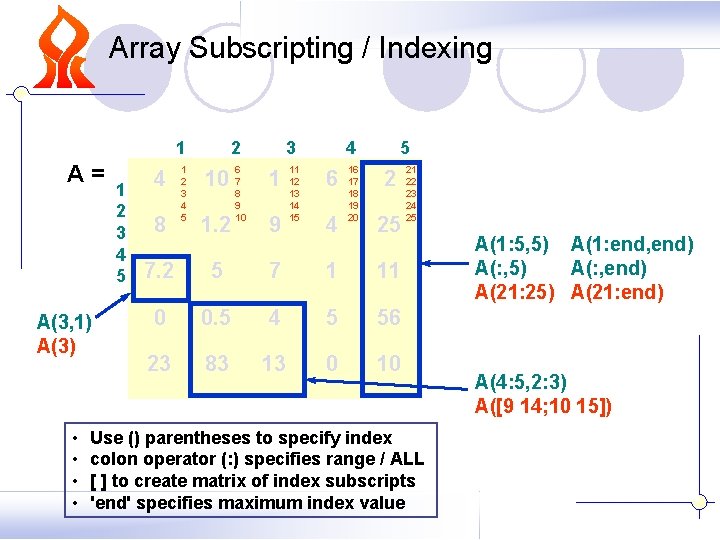
Array Subscripting / Indexing A= A(3, 1) A(3) • • 1 2 3 4 5 4 8 1 2 3 4 5 10 7 1 1. 2 9 6 8 9 10 3 11 12 13 14 15 4 6 4 16 17 18 19 20 5 2 25 7. 2 5 7 1 11 0 0. 5 4 5 56 23 83 13 0 10 21 22 23 24 25 Use () parentheses to specify index colon operator (: ) specifies range / ALL [ ] to create matrix of index subscripts 'end' specifies maximum index value A(1: 5, 5) A(1: end, end) A(: , 5) A(: , end) A(21: 25) A(21: end)’ A(4: 5, 2: 3) A([9 14; 10 15])

Matrix examples: >> a=[1 2; 3 4] a = 1 2 3 4 >> a(1, 4)=5 % auto enlarging a = 1 2 0 5 3 4 0 0 >> a(: , 3)=[4; 4] a = 1 2 4 5 3 4 4 0 >> b=a(: , 4: -1: 1) b = 5 4 2 1 0 4 4 3 >> b(6) % columnwise unraveling ans = 4 >> b(: ) % columnwise unraveling ans = 5 0 4 4 2 4 1 3 >> b(1, : )=[] % erasing a row b = 0 4 4 3

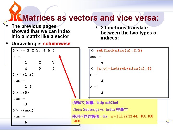
Matrices as vectors and vice versa: • The previous pages showed that we can index into a matrix like a vector • Unraveling is columnwise • 2 functions translate between the two types of indices: >> a=[1 2 3; 4 5 6] >> sub 2 ind(size(a), 2, 3) a = ans = 1 2 3 4 5 6 >> a(1: 2) 6 >> [r, c]=ind 2 sub(size(a), 4) r = ans = 1 4 >> a(5) ans = 3 2 c = 2 (測試? !)建議 – help sub 2 ind >> a(end) Note: Subscript vs. index 差異? ? ans = 使用不同的數值，Ex: a = [ 11 22 33 44; 100: 100 : 400] 6

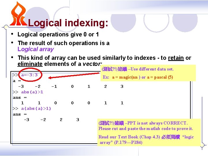
Logical indexing: • • Logical operations give 0 or 1 • This kind of array can be used similarly to indexes - to retain or eliminate elements of a vector: The result of such operations is a Logical array (測試? !)建議 –Use different data set. >> a=-3: 3 a = -3 -2 -1 >> abs(a)>1 ans = 1 1 0 >> a(abs(a)>1) ans = -3 -2 2 Ex: a = magic(nn ) or a = pascal (5) 0 1 2 3 0 0 1 1 3 (測試? !)建議 –PPT is not always CORRECT. Please cut and paste the matlab code to prove it. Read our Text Book (Chap 4. 3) 必須閱讀 “logic array” (P. 179—P 184)

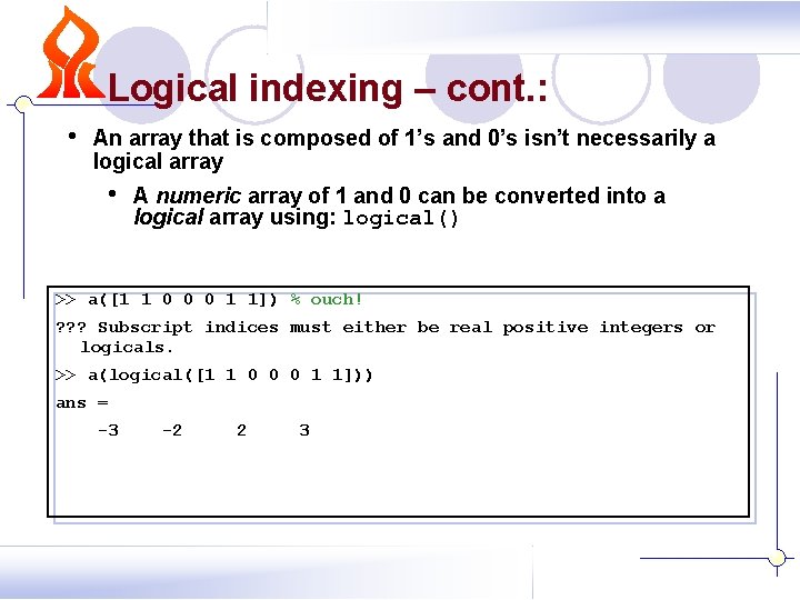
Logical indexing – cont. : • An array that is composed of 1’s and 0’s isn’t necessarily a logical array • A numeric array of 1 and 0 can be converted into a logical array using: logical() >> a([1 1 0 0 0 1 1]) % ouch! ? ? ? Subscript indices must either be real positive integers or logicals. >> a(logical([1 1 0 0 0 1 1])) ans = -3 -2 2 3

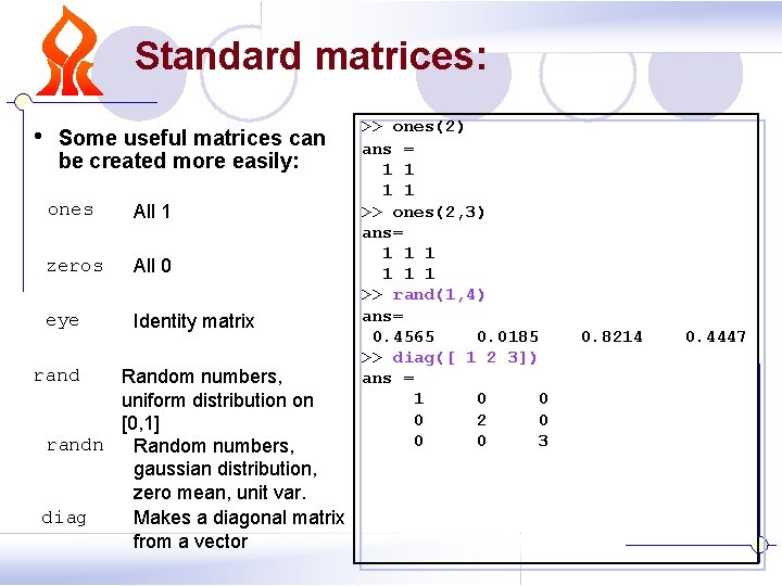
Standard matrices: • Some useful matrices can be created more easily: ones All 1 zeros All 0 eye Identity matrix rand Random numbers, uniform distribution on [0, 1] randn Random numbers, gaussian distribution, zero mean, unit var. diag Makes a diagonal matrix from a vector >> ones(2) ans = 1 1 >> ones(2, 3) ans= 1 1 1 >> rand(1, 4) ans= 0. 4565 0. 0185 >> diag([ 1 2 3]) ans = 1 0 0 0 2 0 0 0 3 0. 8214 0. 4447

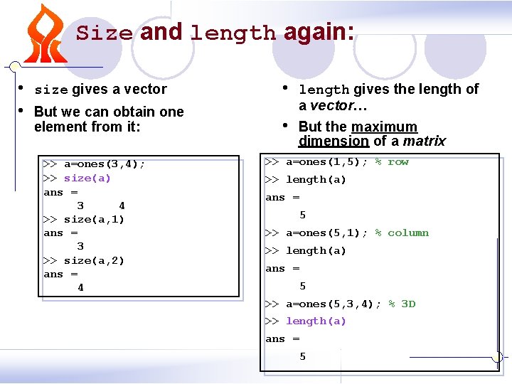
Size and length again: • • size gives a vector • But we can obtain one element from it: length gives the length of a vector… • But the maximum dimension of a matrix >> a=ones(3, 4); >> size(a) ans = 3 4 >> size(a, 1) ans = 3 >> size(a, 2) ans = 4 >> a=ones(1, 5); % row >> length(a) ans = 5 >> a=ones(5, 1); % column >> length(a) ans = 5 >> a=ones(5, 3, 4); % 3 D >> length(a) ans = 5

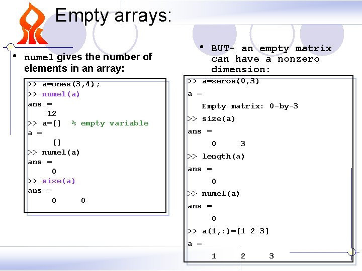
Empty arrays: • numel gives the number of elements in an array: >> a=ones(3, 4); >> numel(a) ans = 12 >> a=[] % empty variable a = [] >> numel(a) ans = 0 >> size(a) ans = 0 0 • BUT- an empty matrix can have a nonzero dimension: >> a=zeros(0, 3) a = Empty matrix: 0 -by-3 >> size(a) ans = 0 3 >> length(a) ans = 0 >> numel(a) ans = 0 >> a(1, : )=[1 2 3] a = 1 2 3

Rearranging the dimensions: • reshape takes the elements of an array and rearranges with new dimensions: >> a=1: 10; % 10 elements >> reshape(a, 2, 5) % 10 elements! ans = 1 3 5 7 9 2 4 6 8 10 >> reshape(a, 5, 2) % 10 elements! ans = 1 6 2 7 3 8 4 9 5 10 • repmat repeats an array (測試? !) >> a=[1 2; 3 4]; >> repmat(a, 1, 2) ans = 1 2 3 4 >> repmat(a, [1 2]) % same ans = 1 2 3 4 >> repmat(a, 2) % ‘ 2’ is extended ans = 1 2 1 2 3 4 3 4

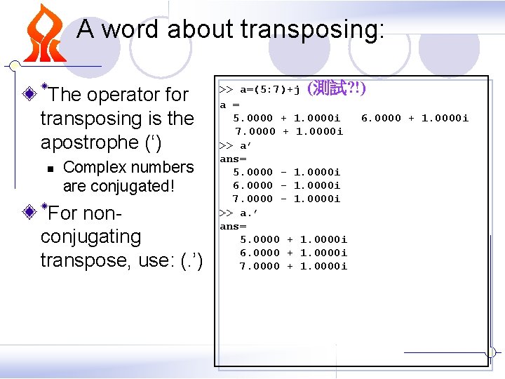
A word about transposing: The operator for transposing is the apostrophe (‘) n Complex numbers are conjugated! For nonconjugating transpose, use: (. ’) >> a=(5: 7)+j (測試? !) a = 5. 0000 + 1. 0000 i 6. 0000 + 1. 0000 i 7. 0000 + 1. 0000 i >> a’ ans= 5. 0000 - 1. 0000 i 6. 0000 - 1. 0000 i 7. 0000 - 1. 0000 i >> a. ’ ans= 5. 0000 + 1. 0000 i 6. 0000 + 1. 0000 i 7. 0000 + 1. 0000 i

Array sorting Matrices: each column is sorted separately: • Vectors: >> x=randperm(6) x = 2 4 3 6 5 1 >> xs=sort(x) %ascending xs = 1 2 3 4 5 6 >> [xs, ixs]=sort(x) %ascending xs = 1 2 3 4 5 6 ixs = 6 1 3 2 5 4 >> m=[randperm(4); randperm(4)] m = 1 4 3 2 2 3 4 1 1 2 4 3 >> [sm, ism]=sort(m) sm = 1 2 3 1 1 3 4 2 2 4 4 3 1 2 3 2 2 1 3 3 ism = Note: randperm(n) gives a random permutation of the integers from 1 to n (測試? !)建議改用m = magic(4) and test [sm, ism] =sort(m) to find what it is.

Array sorting – contd. • Sorting all columns based on only one: >> m %% use m=magic(4) to test it again m = 1 4 3 2 2 3 4 1 1 2 4 3 >> [tmp, ind]=sort(m(: , 2)); >> % based on 2'nd column >> m(ind, : ) ans = 1 2 4 3 2 3 4 1 1 4 3 2 • Sort rows: >> [sm, ism]=sort(m, 2) % add a dimension sm = 1 2 3 4 1 4 3 2 4 1 2 3 1 2 4 3 ism = (測試? !)建議改用m = magic(4) and test [sm, ism] =sort(m) to find what it is.

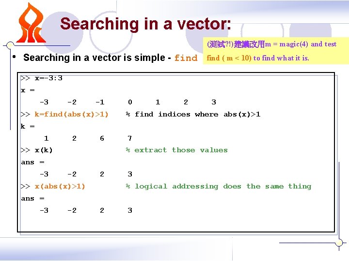
Searching in a vector: (測試? !)建議改用m = magic(4) and test • Searching in a vector is simple - find ( m < 10) to find what it is. >> x=-3: 3 x = -3 -2 -1 >> k=find(abs(x)>1) 0 1 2 3 % find indices where abs(x)>1 k = 1 2 6 >> x(k) 7 % extract those values ans = -3 -2 2 >> x(abs(x)>1) 3 % logical addressing does the same thing ans = -3 -2 2 3

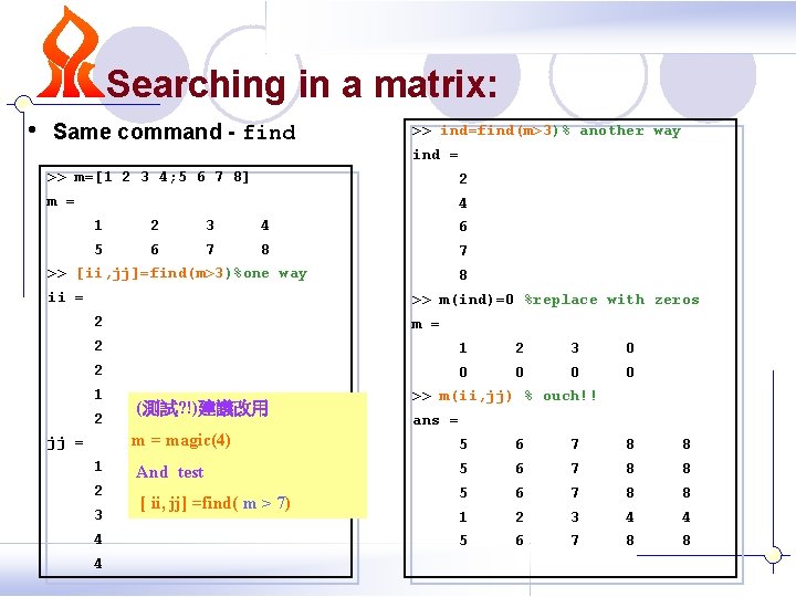
Searching in a matrix: • Same command - find >> ind=find(m>3)% another way ind = >> m=[1 2 3 4; 5 6 7 8] 2 m = 4 1 2 3 4 6 5 6 7 8 7 >> [ii, jj]=find(m>3)%one way ii = 8 >> m(ind)=0 %replace with zeros 2 m = 2 1 2 3 0 2 0 0 1 2 jj = 1 2 3 4 4 (測試? !)建議改用 >> m(ii, jj) % ouch!! ans = magic(4) 5 6 7 8 8 And test 5 6 7 8 8 1 2 3 4 4 5 6 7 8 8 [ ii, jj] =find( m > 7)

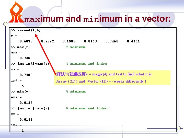
maximum and minimum in a vector: >> v=rand(1, 6) v = 0. 6038 0. 2722 >> max(v) 0. 1988 0. 0153 0. 7468 0. 4451 % maximum ans = 0. 7468 >> [mx, ind]=max(v) % maximum and index mx = 0. 7468 ind = (測試? !)建議改用v = magic(4) and test to find what it is. Array ( 2 D ) and Vector (1 D) --- works differently ! 5 >> min(v) % minimum ans = 0. 0153 >> [mn, ind]=min(v) mn = 0. 0153 ind = 4 % minimum and index

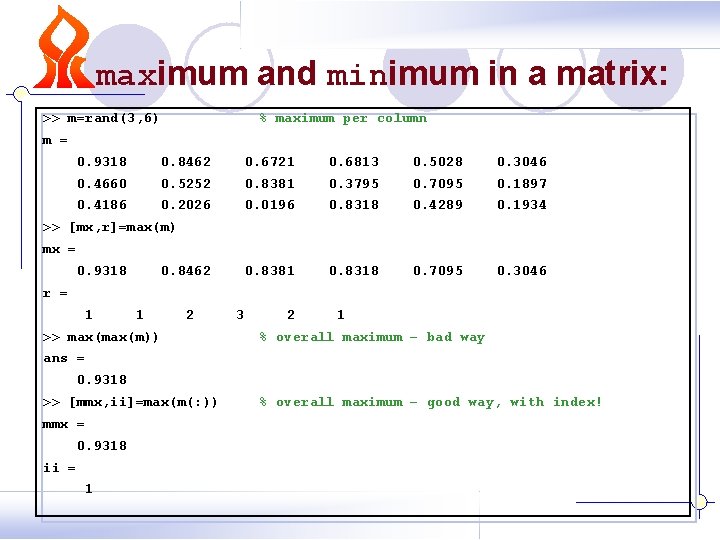
maximum and minimum in a matrix: >> m=rand(3, 6) % maximum per column m = 0. 9318 0. 8462 0. 6721 0. 6813 0. 5028 0. 3046 0. 4660 0. 5252 0. 8381 0. 3795 0. 7095 0. 1897 0. 4186 0. 2026 0. 0196 0. 8318 0. 4289 0. 1934 0. 8381 0. 8318 0. 7095 0. 3046 >> [mx, r]=max(m) mx = 0. 9318 0. 8462 r = 1 1 2 >> max(m)) 3 2 1 % overall maximum – bad way ans = 0. 9318 >> [mmx, ii]=max(m(: )) mmx = 0. 9318 ii = 1 % overall maximum – good way, with index!

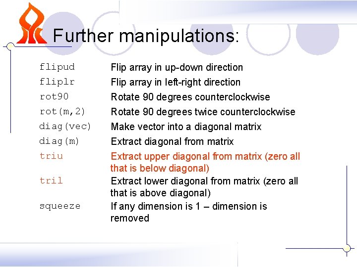
Further manipulations: flipud Flip array in up-down direction fliplr rot 90 rot(m, 2) diag(vec) diag(m) triu Flip array in left-right direction Rotate 90 degrees counterclockwise Rotate 90 degrees twice counterclockwise Make vector into a diagonal matrix Extract diagonal from matrix Extract upper diagonal from matrix (zero all that is below diagonal) Extract lower diagonal from matrix (zero all that is above diagonal) If any dimension is 1 – dimension is removed tril squeeze

Array math in Matlab Linear algebra vs. simple algebra When performing mathematical operations between arrays in Matlab – how do we determine what rules will be used? Matlab has a set of rules that is generally simple and easy to follow Let’s examine the possible cases:

Scalar/Matrix math: Scalar expansion >> w=[1 2; 3 4] + 5 1 2 = + 5 3 4 1 2 5 5 = + 3 4 5 5 6 7 = 8 9 >> w=[1 2; 3 4] + 5 w = 6 7 8 9 (測試? !)建議 –PPT is not always CORRECT. Please cut and paste the matlab code to prove it. Generally this works for + - * / ^ …

Similarly: >> w=[1 2; 3 4] + 5 w = 6 7 8 9 >> w=5 * [1 2; 3 4] w = 6 7 8 9 >> w=[1 2; 3 4] / 5 w = 0. 2 0. 4 0. 6 0. 8 BUT: >> w=5 / [1 2; 3 4] ? ? ? Error using ==> mrdivide Matrix dimensions must agree. To resolve this we have to go a bit further… (測試? !)建議 –PPT is not always CORRECT. Please cut and paste the matlab code to prove it.

Simple Matrix/Matrix math: • Performing calculations element by element: • • • Matrices must be the same size With + and – there is no ambiguity With other operators – add a dot: . *. /. ^ etc. >> w=[1 2; 3 4] + [5 5; 5 5] 6 7 = 8 9 >> w=[1 2; 3 4]. * [5 5; 5 5] 5 10 15 20 = … and to address the problem on the previous slide: >> w=5. / [1 2; 3 4] 5 2. 5 1. 6667 1. 25

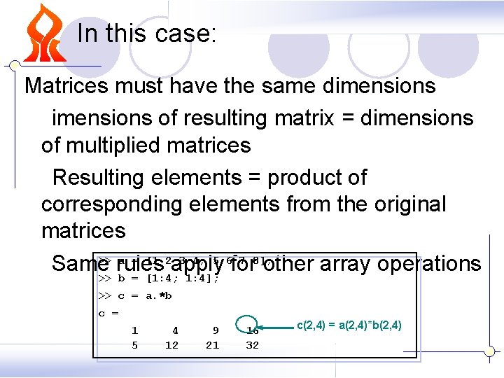
In this case: Matrices must have the same dimensions of resulting matrix = dimensions of multiplied matrices Resulting elements = product of corresponding elements from the original matrices >> a = [1 2 3 4; 5 6 7 8]; Same rules apply for other array operations >> b = [1: 4; 1: 4]; >> c = a. *b c = 1 5 4 12 9 21 16 32 c(2, 4) = a(2, 4)*b(2, 4)

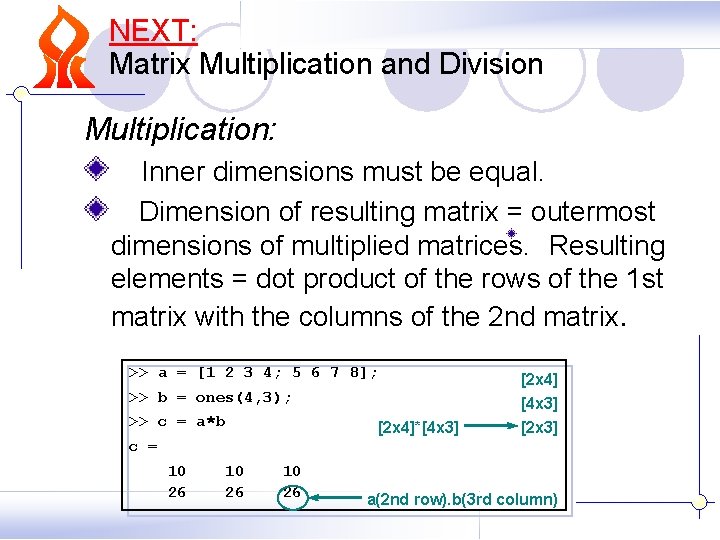
NEXT: Matrix Multiplication and Division Multiplication: Inner dimensions must be equal. Dimension of resulting matrix = outermost dimensions of multiplied matrices. Resulting elements = dot product of the rows of the 1 st matrix with the columns of the 2 nd matrix. >> a = [1 2 3 4; 5 6 7 8]; >> b = ones(4, 3); >> c = a*b [2 x 4]*[4 x 3] [2 x 4] [4 x 3] [2 x 3] c = 10 26 a(2 nd row). b(3 rd column)

Division (solving equations): using “Left Division” To Solve the set of simultaneous equations: we need to calculate: Ax = b >> A = [-1 1 2; 3 -1 1; -1 3 4]; -x 1 + x 2 + 2 x 3 = 2 >> b = [2; 6; 4]; 3 x 1 - x 2 + x 3 = 6 x = >> x = inv(A)*b 1. 0000 -x 1 + 3 x 2 + 4 x 3 = 4 -1. 0000 2. 0000 >> x = Ab x = 1. 0000 -1. 0000 2. 0000

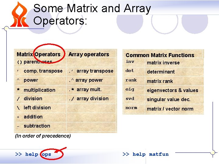
Some Matrix and Array Operators: Matrix Operators Array operators Common Matrix Functions () parentheses inv matrix inverse ’ comp. transpose . ’ array transpose determinant ^ power . ^ array power rank matrix rank * multiplication . * array mult. eigenvectors & values / division . / array division svd singular value dec. norm matrix / vector norm left division + addition - subtraction (In order of precedence) >> help ops >> help matfun

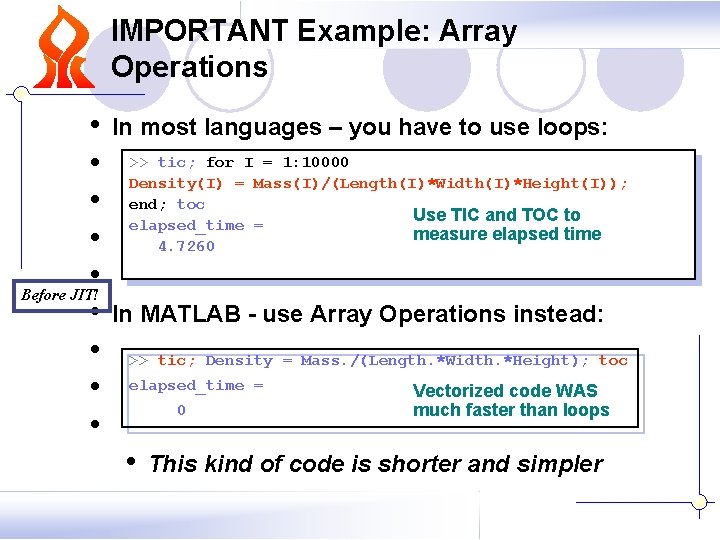
IMPORTANT Example: Array Operations • • • Before JIT! • • In most languages – you have to use loops: >> tic; for I = 1: 10000 Density(I) = Mass(I)/(Length(I)*Width(I)*Height(I)); end; toc Use TIC and TOC to elapsed_time = measure elapsed time 4. 7260 In MATLAB - use Array Operations instead: >> tic; Density = Mass. /(Length. *Width. *Height); toc elapsed_time = 0 • Vectorized code WAS much faster than loops This kind of code is shorter and simpler

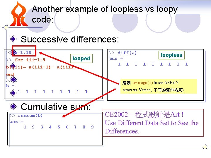
Another example of loopless vs loopy code: Successive differences: >> a=1: 10; >> diff(a) loopless ans = looped >> for iii=1: 9 1 1 1 1 1 b(iii)= a(iii+1)a(iii); end >> b 建議: a= magic(5) to see ARRAY b = Array vs. Vector ( 不同的運作格局) 1 1 1 1 1 Cumulative sum: >> cumsum(b) ans = 1 2 3 4 5 6 7 8 9 CE 2002—程式設計是Art ! Use Different Data Set to See the Differences.

Summary: Arrays are very easy to use in MATLAB No declarations are necessary, and array dimensions can be modified dynamically Manipulating and indexing into arrays is very powerful, and can be complicated at times Arrays can be sorted and searched easily Math with arrays can be performed either element by element, or as defined by the 建議 –The PPT is not always CORRECT. Please cut and paste the matlab code to prove it. rules of linear algebra Last Note: Carefully play every CE 2002—PRn. SWF (Flash Movie) to learn more. 01/17/07