LESSON 4 5 Graphing Other Trigonometric Functions FiveMinute

LESSON 4– 5 Graphing Other Trigonometric Functions

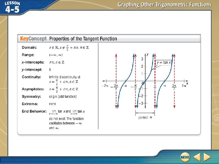
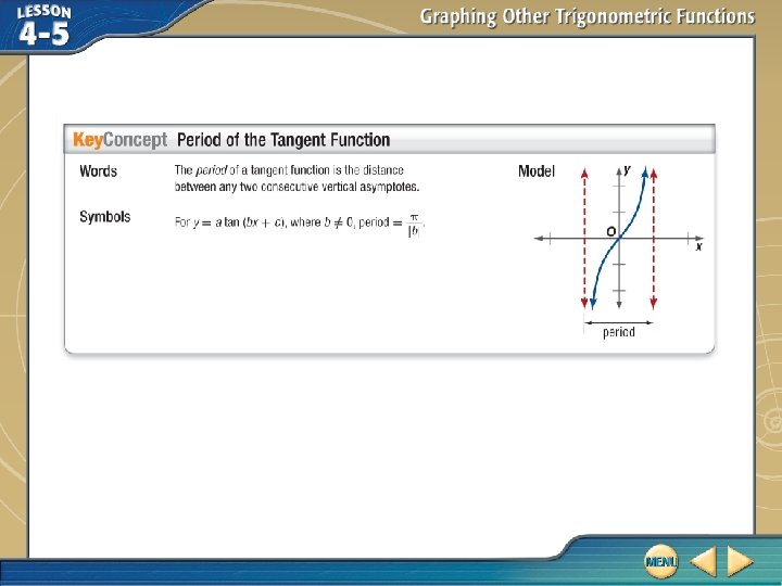
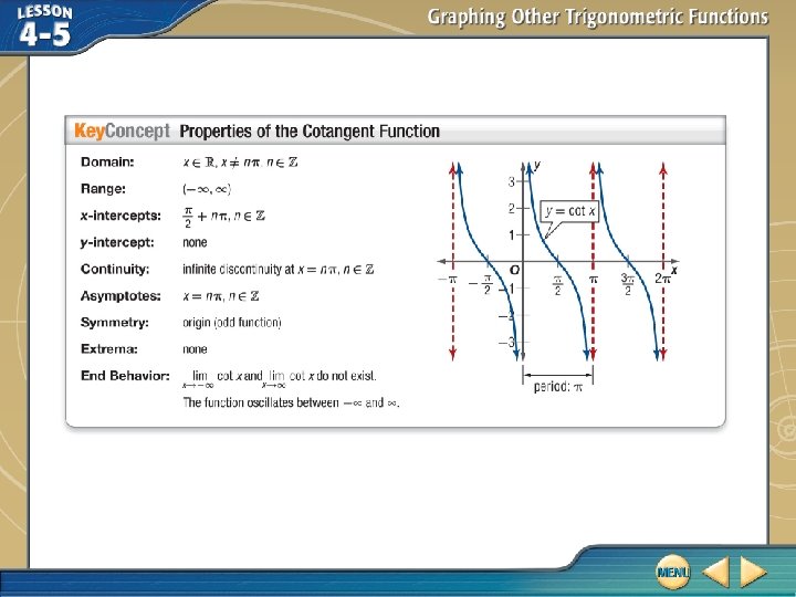
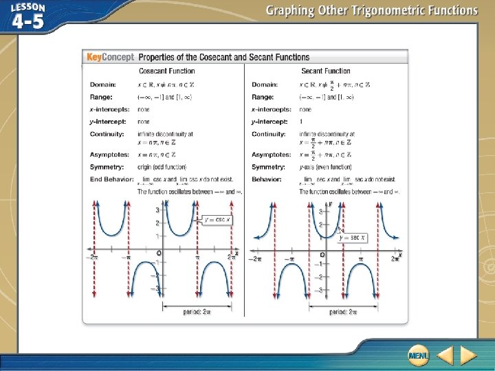
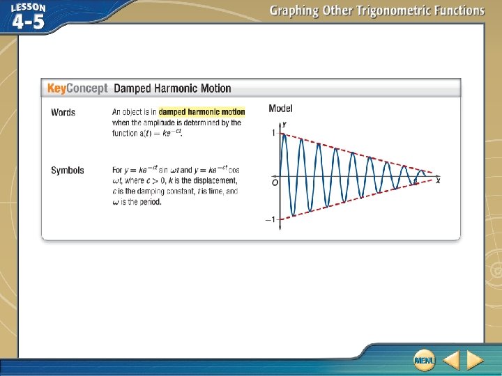
Five-Minute Check (over Lesson 4 -4) TEKS Then/Now New Vocabulary Key Concept: Properties of the Tangent Function Key Concept: Period of the Tangent Function Example 1: Graph Horizontal Dilations of the Tangent Function Example 2: Graph Reflections and Translations of the Tangent Function Key Concept: Properties of the Cotangent Function Example 3: Sketch the Graph of a Cotangent Function Key Concept: Properties of the Cosecant and Secant Functions Example 4: Sketch Graphs of Cosecant and Secant Functions Example 5: Sketch Damped Trigonometric Functions Key Concept: Damped Harmonic Motion Example 6: Real-World Example: Damped Harmonic Motion

Over Lesson 4 -4 A. Describe how the graphs of f (x) = sin x and g (x) = 2 sin x are related. Then find the amplitude and period of g (x). A. The graph of g (x) is the graph of f (x) expanded horizontally. amplitude = 2, period = 24. B. The graph of g (x) is the graph of f (x) compressed horizontally. amplitude = 1, period = π. C. The graph of g (x) is the graph of f (x) expanded vertically. amplitude = 2, period = 2π. D. The graph of g (x) is the graph of f (x) compressed vertically. amplitude = 0. 5, period = 2π.

Over Lesson 4 -4 B. Sketch the graphs of f (x) = sin x and g (x) = 2 sin x on the same coordinate axes. A. C. B. D.

Over Lesson 4 -4 A. State the amplitude, period, frequency, phase shift, and vertical shift of A. amplitude = 2; period = 2π; frequency = ; phase shift = B. amplitude = 1; period = π; frequency = ; phase shift = C. amplitude = 2; period = 2π; frequency = ; phase shift = D. amplitude = frequency = period = ; ; phase shift = ;

Over Lesson 4 -4 B. Graph two periods of A. C. B. D.

Over Lesson 4 -4 Write a sinusoidal function that can be used to model the initial behavior of a sound wave with a frequency of 820 hertz and an amplitude of 0. 35. A. y = 0. 35 sin 820 t B. y = 0. 35 sin 410πt C. y = 0. 35 sin 820πt D. y = 0. 35 sin 1640πt

Targeted TEKS P. 2(F) Graph exponential logarithmic rational, polynomial, power, trigonometric, inverse trigonometric, and piecewise defined functions, including step functions. P. 2(I) Determine and analyze the key features of exponential, logarithmic, rational, polynomial, power, trigonometric, inverse trigonometric, and piecewise defined functions, including step functions such as domain, range, symmetry, relative maximum, relative minimum, zeros, asymptotes, and intervals over which the function is increasing or decreasing. Also addresses P. 4(F). Mathematical Processes P. 1(A), P. 1(F)

You analyzed graphs of trigonometric functions. (Lesson 4 -4) • Graph tangent and reciprocal trigonometric functions. • Graph damped trigonometric functions.

• damped trigonometric function • damping factor • damped oscillation • damped wave • damped harmonic motion

Graph Horizontal Dilations of the Tangent Function Locate the vertical asymptotes, and sketch the graph of y = tan . The graph of y = tan is the graph of y = tan x expanded horizontally. The period is or 3. Find two consecutive vertical asymptotes by solving bx + c = – and bx + c = .

Graph Horizontal Dilations of the Tangent Function Create a table listing key points, including the x-intercept, that are located between the two vertical asymptotes at

Graph Horizontal Dilations of the Tangent Function Sketch the curve through the indicated key points for the function. Then sketch one cycle to the left on and one cycle to the right on .

Graph Horizontal Dilations of the Tangent Function Answer:

A. Locate the vertical asymptotes of y = tan 4 x. A. vertical asymptotes: , n is an odd integer B. vertical asymptotes: , n is an odd integer C. vertical asymptotes: , n is an integer D. vertical asymptotes: , n is an odd integer

B. Sketch the graph of y = tan 4 x. A. C. B. D.

Graph Reflections and Translations of the Tangent Function A. Locate the vertical asymptotes, and sketch the graph of The graph of y = –tan . is the graph of y = tan x expanded horizontally and then reflected in the x-axis. The period is asymptotes. . Find two consecutive vertical

Graph Reflections and Translations of the Tangent Function Multiply. Create a table listing key points, including the x-intercept, that are located between the two vertical asymptotes at x = – 2 and x = 2.

Graph Reflections and Translations of the Tangent Function Sketch the curve through the indicated key points for the function. Then repeat the pattern for one cycle to the left and right of the first curve. Answer:

Graph Reflections and Translations of the Tangent Function B. Locate the vertical asymptotes, and sketch the graph of . The graph of y = –tan shifted is the graph of y = tan x to the left and then reflected in the x-axis. The period is asymptotes. or π. Find two consecutive vertical

Graph Reflections and Translations of the Tangent Function Subtract. Create a table listing key points, including the x-intercept, that are located between the two vertical asymptotes at x = – and x = 0.

Graph Reflections and Translations of the Tangent Function Sketch the curve through the indicated key points for the function. Then sketch one cycle to the left and right. Answer:

Locate the vertical asymptotes of the graph of y = – tan(3 x + π). A. vertical asymptotes: n is an odd integer B. vertical asymptotes: n is an integer C. vertical asymptotes: n is an odd integer D. vertical asymptotes: n is an integer

Sketch the Graph of a Cotangent Function Locate the vertical asymptotes, and sketch the graph of y = cot 2 x. The graph of y = cot 2 x is the graph of y = cot x compressed horizontally. The period is or . Find two consecutive vertical asymptotes. 2 x + 0 = 0 x =0 b = 2, c = 0 Simplify. 2 x + 0 = x=

Sketch the Graph of a Cotangent Function Create a table listing key points, including the x-intercept, that are located between the two vertical asymptotes at x = 0 and x =.

Sketch the Graph of a Cotangent Function Following the same guidelines that you used for the tangent function, sketch the curve through the indicated key points that you found. Then sketch one cycle to the left and right of the first curve. Answer:

A. Locate the vertical asymptotes of A. vertical asymptotes: n is an odd integer B. vertical asymptotes: n is an integer C. vertical asymptotes: x = nπ, n is an odd integer D. vertical asymptotes: x = nπ, n is an integer

B. Sketch the graph of A. C. B. D.

Sketch Graphs of Cosecant and Secant Functions A. Locate the vertical asymptotes, and sketch the graph of y = –sec 2 x. The graph of y = –sec 2 x is the graph of y = sec x compressed horizontally and then reflected in the x-axis. The period is or . Two vertical asymptotes occur when bx + c = and bx + c = Therefore, two asymptotes are 2 x + 0 = or x = – and 2 x + 0 = or x = . .

Sketch Graphs of Cosecant and Secant Functions Create a table listing key points that are located between the asymptotes at x = and x = .

Sketch Graphs of Cosecant and Secant Functions Graph one cycle on the interval. Then sketch one cycle to the left and right. Answer:

Sketch Graphs of Cosecant and Secant Functions B. Locate the vertical asymptotes, and sketch the graph of . The graph of y = csc shifted is the graph of y = csc x units to the left. The period is or 2. Two vertical asymptotes occur when bx + c = – and bx + c = . Therefore, two asymptotes are x + or x = and x + = or x = . = –

Sketch Graphs of Cosecant and Secant Functions Create a table listing key points, including the relative maximum and minimum, that are located between the two vertical asymptotes at x = and x = .

Sketch Graphs of Cosecant and Secant Functions Sketch the curve through the indicated key points for the function. Then sketch one cycle to the left and right. Answer:

A. Locate the vertical asymptotes of y = csc A. x = nπ, n is an odd integer B. n is an integer C. n is an odd integer D. x = nπ, n is an integer

B. Sketch the graph of y = csc A. C. B. D.

Sketch Damped Trigonometric Functions A. Identify the damping factor f (x) of . Then use a graphing calculator to sketch the graphs of f (x), –f (x), and the given function in the same viewing window. Describe the behavior of the graph. The function y = y= is the product of the functions and y = sin x, so f(x) = .

Sketch Damped Trigonometric Functions The amplitude of the function is decreasing as x approaches 0 from both directions.

Sketch Damped Trigonometric Functions Answer: f (x) = ; The amplitude is decreasing as x approaches 0 from both directions.

Sketch Damped Trigonometric Functions B. Identify the damping factor f (x) of y = x 2 cos 3 x. Then use a graphing calculator to sketch the graphs of f (x), –f (x), and the given function in the same viewing window. Describe the behavior of the graph. The function y = x 2 cos 3 x is the product of the functions y = x 2 and y = cos 3 x. Therefore, the damping factor is f (x) = x 2. The amplitude is decreasing as x approaches 0 from both directions.

Sketch Damped Trigonometric Functions Answer: f (x) = x 2; The amplitude is decreasing as x approaches 0 from both directions.

Identify the damping factor f (x) of y = 4 x sin x. A. f (x) = 4 x B. f (x) = C. f (x) = sin x D. f (x) = 4 x sin x

Damped Harmonic Motion A. MUSIC A guitar string is plucked at a distance of 0. 95 centimeter above its rest position, then released, causing a vibration. The damping constant for the string is 1. 3, and the note produced has a frequency of 200 cycles per second. Write a trigonometric function that models the motion of the string. The maximum displacement of the string occurs when t = 0, so y = ke–ct cos t can be used to model the motion of the string because the graph of y = cos wt has a y-intercept other than 0.

Damped Harmonic Motion The maximum displacement occurs when the string is plucked 0. 95 centimeter. The total displacement is the maximum displacement M minus the minimum displacement m, so k = M – m = 0. 95 – 0 or 0. 95 cm. You can use the value of the frequency to find w. = frequency Multiply each side by 2π.

Damped Harmonic Motion Write a function using the values of k, w, and c. y = 0. 95 e– 1. 3 t cos 400πt is one model that describes the motion of the string. Sample Answer: y = 0. 95 e– 1. 3 t cos 400πt

Damped Harmonic Motion B. MUSIC A guitar string is plucked at a distance of 0. 95 centimeter above its rest position, then released, causing a vibration. The damping constant for the string is 1. 3, and the note produced has a frequency of 200 cycles per second. Determine the amount of time t that it takes the string to be damped so that – 0. 38 ≤ y ≤ 0. 38. Use a graphing calculator to determine the value of t when the graph of y = 0. 95 e– 1. 3 t cos 400πt is oscillating between y = – 0. 38 and y = 0. 38.

Damped Harmonic Motion From the graph, you can see that it takes approximately 0. 7 second for the graph of y = 0. 95 e– 1. 3 t cos 400πt to oscillate within the interval – 0. 38 ≤ y ≤ 0. 38. Answer: about 0. 7 second

MUSIC Suppose another string on the guitar was plucked 0. 3 centimeter above its rest position with a frequency of 64 cycles per second a damping constant of 1. 4. Write a trigonometric function that models the motion of the string y as a function of time t. A. y = 0. 3 e– 2. 8 t cos 64πt B. y = 0. 6 e– 0. 07 t cos 32πt C. y = 0. 15 e– 5. 6 t cos 256πt D. y = 0. 3 e– 1. 4 t cos 128πt

LESSON 4– 5 Graphing Other Trigonometric Functions