Lesson 3 Overview Descriptive Procedures PRINT MEANS UNIVARIATE

Lesson 3 Overview • Descriptive Procedures – PRINT, MEANS, UNIVARIATE, SGPLOT • Controlling SAS Output • Program 3 in course notes • LSB: See syllabus

Descriptive Procedures In SAS

Syntax for Procedures PROCNAME DATA=datasetname <options> ; substatements/<options> ; The WHERE statement is a useful substatement available to all procedures. PROC FREQ DATA=demo ; TABLES marstat; WHERE state = 'MN'; RUN;

Data Layout of tomhs. dat TOMHS Data Dictionary (website) Variable Type Len Pos Inform Description PTID Char 10 1 $10. Patient ID CLINIC Char 1 12 $1. Clinical center RANDDATE Num 6 14 mmddyy 10. Randdate SBPBL Num 3 115 3. SBP at baseline DATA tomhs; INFILE ‘folderpathtomhs. dat'; INPUT @1 ptid $10. @12 clinic $1. @14 randdate mmddyy 10. @115 sbpbl 3. ; Note: You can give any legal variable name.

Program 3 DATA weight; INFILE ‘C: SAS_Filestomhs. dat' ; INPUT @1 ptid $10. @12 clinic $1. @30 sex 1. @58 height 4. @85 weight 5. ; * Create new variables here; bmi = (weight*703. 0768)/(height*height); * BMI is calculated in kg/m 2; RUN;

SAS Data Step: Build in Loop DATA weight; INFILE ‘C: SAS_Filestomhs. dat'; * EOF then stop INPUT @1 ptid $10. Gets @12 clinic $1. repeated for @30 sex $1. @58 height 4. each data @85 weight 5. ; row bmi = (weight*703. 0768)/(height*height); OUTPUT; * Inserted by SAS RUN;

PROC PRINT DATA = weight (OBS=5); TITLE 'Proc Print: Five observations from the TOMHS Study'; RUN; PROC MEANS DATA = weight; VAR height weight bmi; TITLE 'Proc Means Example 1'; RUN; PROC MEANS DATA = weight MEAN MEDIAN STD MAXDEC=2; VAR height weight bmi; TITLE 'Proc Means Example 2 (specifying options)'; RUN; Page 258 of Little SAS Book (5 th edition) Also see online help under proc means

Proc Print: Five observations from the TOMHS Study Obs 1 2 3 4 5 ptid C 03615 B 00979 B 00644 D 01348 A 01088 clinic sex height weight bmi C B B D A 1 1 1 71. 5 69. 5 60. 0 71. 5 72. 0 205. 5 247. 3 138. 5 205. 5 244. 8 28. 2620 35. 9963 27. 0489 28. 2620 33. 2008 Proc Means Example 1 The MEANS Procedure Variable N Mean Std Dev Minimum Maximum -------------------------------------height 100 68. 0750000 3. 8536189 58. 0000000 77. 0000000 weight 100 191. 7560000 34. 5107254 128. 5000000 279. 3000000 bmi 100 28. 9808397 3. 9911476 21. 4572336 37. 5178852 -------------------------------------

Proc Means Example 2 (specifying options) The MEANS Procedure Variable Mean Median Std Dev ----------------------------height 68. 08 67. 50 3. 85 weight 191. 76 192. 65 34. 51 bmi 28. 98 28. 02 3. 99 ----------------------------

OMITTING RUN STATEMENTS PROC PRINT DATA = weight (OBS=5); PROC MEANS DATA = weight; VAR height weight bmi; PROC MEANS DATA = weight MEAN MEDIAN; VAR height weight bmi; THIS CODE WILL RUN THE FIRST TWO PROCEDURES BUT NOT THE LAST

PROC MEANS DATA = weight N MEAN STD MAXDEC=2 ; CLASS clinic; VAR height weight bmi; TITLE 'Proc Means Example 3 (Using a CLASS statement)'; RUN; N clinic Obs Variable N Mean Std Dev -----------------------------A 18 height 18 67. 89 3. 04 weight 18 192. 73 37. 68 bmi 18 29. 24 4. 50 B 29 height weight bmi 29 29 29 67. 76 185. 58 28. 39 4. 76 34. 00 4. 22 C 36 height weight bmi 36 36 36 69. 08 202. 91 29. 76 3. 36 33. 74 3. 62 D 17 height 17 66. 68 3. 61 weight 17 177. 65 28. 05 bmi 17 28. 06 3. 79 -----------------------------

* Adding WAYS statement to get totals and by clinic; PROC MEANS DATA = weight N MEAN STD MAXDEC=2; CLASS clinic; VAR height weight bmi; WAYS 0 1 ; RUN; N Obs Variable N Mean Std Dev -----------------------------100 height 100 68. 08 3. 85 weight 100 191. 76 34. 51 bmi 100 28. 98 3. 99 N clinic Obs Variable N Mean Std Dev -----------------------------A 18 height 18 67. 89 3. 04 weight 18 192. 73 37. 68 bmi 18 29. 24 4. 50 B 29 height weight bmi 29 29 29 67. 76 185. 58 28. 39 4. 76 34. 00 4. 22 C 36 height weight bmi 36 36 36 69. 08 202. 91 29. 76 3. 36 33. 74 3. 62 D 17 height weight bmi 17 17 17 66. 68 177. 65 28. 06 3. 61 28. 05 3. 79

* Could also sort the data by clinic and then use BY statement; PROC SORT data=weight; BY clinic; PROC MEANS DATA = weight N MEAN STD MAXDEC=2 ; VAR height weight bmi; TITLE 'Proc Means Example 4 (Using a BY statement)'; BY clinic; RUN; clinic=A Partial Output Variable N Mean Std Dev ƒƒƒƒƒƒƒƒƒƒƒƒƒƒƒƒƒƒƒƒ height 18 67. 89 3. 04 weight 18 192. 73 37. 68 bmi 18 29. 24 4. 50 ƒƒƒƒƒƒƒƒƒƒƒƒƒƒƒƒƒƒƒƒ clinic=B Variable N Mean Std Dev ƒƒƒƒƒƒƒƒƒƒƒƒƒƒƒƒƒƒƒƒ height 29 67. 76 4. 76 weight 29 185. 58 34. 00 bmi 29 28. 39 4. 22 ƒƒƒƒƒƒƒƒƒƒƒƒƒƒƒƒƒƒƒƒ

PROC UNIVARIATE DATA = weight; VAR bmi; ID ptid; TITLE 'Proc Univariate Example 1'; RUN; * Note: PROC UNIVARIATE will give you much output ;

Proc Univariate Example 1 The UNIVARIATE Procedure Variable: bmi Moments N Mean Std Deviation Skewness Uncorrected SS Coeff Variation 100 28. 9808397 3. 99114757 0. 27805446 85565. 9037 13. 7716768 Sum Weights Sum Observations Variance Kurtosis Corrected SS Std Error Mean 100 2898. 08397 15. 9292589 -0. 8987587 1576. 99663 0. 39911476 Basic Statistical Measures Location Mean Median Mode Variability 28. 98084 28. 01524 28. 26198 Std Deviation Variance Range Interquartile Range 3. 99115 15. 92926 16. 06065 6. 68654 Tests for Location: Mu 0=0 Test -Statistic- -----p Value------ Student's t Signed Rank t M S Pr > |t| Pr >= |M| Pr >= |S| 72. 6128 50 2525 <. 0001

Quantiles (Definition 5) Quantile Estimate 100% Max 99% 95% 90% 75% Q 3 50% Median 25% Q 1 10% 5% 1% 0% Min 37. 5179 37. 4385 35. 8871 34. 3378 32. 6299 28. 0152 25. 9433 24. 1495 22. 9373 21. 8969 21. 4572 Extreme Observations ------Lowest------Value 21. 4572 22. 3365 22. 4057 22. 6773 22. 8387 ptid A 00083 C 04206 B 00714 A 00312 B 00262 Obs 64 49 8 21 27 ------Highest-----Value 35. 9963 36. 3726 37. 2037 37. 3592 37. 5179 ptid B 00979 B 03077 A 01166 C 05323 B 02059 Obs 2 67 9 92 25

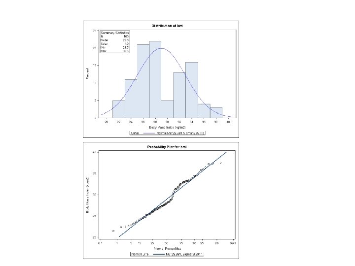
* High resolution graphs can also be produced. The following makes a histogram and normal plot ; ODS GRAPHICS ON; PROC UNIVARIATE DATA = weight; VAR bmi; HISTOGRAM bmi / NORMAL MIDPOINTS=20 to 40 by 2; INSET N = 'N' (5. 0) MEAN = 'Mean' (5. 1) STD = 'Sdev' (5. 1) MIN = 'Min' (5. 1) MAX = 'Max' (5. 1)/ POS=NW HEADER='Summary Statistics'; LABEL bmi = 'Body Mass Index (kg/m 2)'; TITLE 'Histogram of BMI'; PROBPLOT bmi/NORMAL (MU=est SIGMA=est); RUN;

* PROC SGPLOT can do several types of plots PROC SGPLOT; HISTOGRAM bmi; DENSITY bmi/TYPE=NORMAL; DENSITY bmi/TYPE=KERNEL; YAXIS GRID; TITLE ‘HISTOGRAM of BMI'; RUN; HISTOGRAM DENSITY VBOX (HBOX) SCATTER SERIES REG STEP HBAR (VBAR)

* PROC SGPLOT can do several types of plots here a boxplot; PROC SGPLOT; HBOX bmi; XAXIS GRID; TITLE 'Boxplot of BMI'; RUN; 25 th Percentile 75 th Percentile Median

* Using SGPLOT to make side-by-side boxplots; PROC SGPLOT; TITLE "Boxplot of BMI for Men and Women"; HBOX bmi/CATEGORY=sex; RUN;

* Formatting plot; PROC FORMAT; VALUE gender 1=‘Men’ 2=‘Women’; RUN; PROC SGPLOT; TITLE "Boxplot of BMI by Gender"; HBOX bmi/CATEGORY=sex; LABEL sex = ‘Gender’; LABEL bmi = ‘BMI (kg/m 2)’; FORMAT sex gender. ; RUN;

* Using SGPLOT to make scatter plot; PROC SGPLOT; TITLE “Weight vs Height"; SCATTER X=height Y=weight; RUN;

* Using SGPLOT to add regression line; PROC SGPLOT; TITLE “Weight vs Height"; REG X=height Y=weight; RUN;

* With the Output Delivery System you can selectively include only portions of the output; ODS TRACE ON/LISTING; * Lists the names of the pieces of output to the output window (need to add this option); PROC UNIVARIATE DATA = weight ; VAR bmi; TITLE 'Proc Univariate Example 1'; RUN;

Output Window Output Added: ------Name: Moments Label: Moments Template: base. univariate. Moments Path: Univariate. bmi. Moments ------Moments N Mean Std Deviation Skewness Uncorrected SS Coeff Variation 100 28. 9808397 3. 99114757 0. 27805446 85565. 9037 13. 7716768 Sum Weights Sum Observations Variance Kurtosis Corrected SS Std Error Mean 100 2898. 08397 15. 9292589 -0. 8987587 1576. 99663 0. 39911476

* This will restrict output to Basic. Measures and Quantiles tables; ODS TRACE OFF; ODS SELECT Basic. Measures Quantiles; PROC UNIVARIATE DATA = weight ; VAR bmi; RUN;

LIMITING SAS OUTPUT Variable: bmi Basic Statistical Measures Location Mean Median Mode Variability 28. 98084 28. 01524 28. 26198 Std Deviation Variance Range Interquartile Range Quantiles (Definition 5) Quantile 100% Max 99% 95% 90% 75% Q 3 50% Median 25% Q 1 10% 5% 1% 0% Min Estimate 37. 5179 37. 4385 35. 8871 34. 3378 32. 6299 28. 0152 25. 9433 24. 1495 22. 9373 21. 8969 21. 4572 3. 99115 15. 92926 16. 06065 6. 68654

Reading SAS Dataset DATA weight; INFILE ‘C: SAS_Filestomhs. dat' ; INPUT @1 ptid $10. @12 clinic $1. @30 sex $1. @58 height 4. @85 weight 5. ; bmi = (weight*703. 0768)/(height*height); * BMI is calculated in kg/m 2; RUN; DATA weight 2; SET weight (KEEP = ptid clinic sex bmi); WHERE clinic = ‘A’; RUN;