Lesson 3 1 Scatterplots and Correlation Knowledge Objectives

Lesson 3 - 1 Scatterplots and Correlation

Knowledge Objectives • Explain the difference between an explanatory variable and a response variable • Explain what it means for two variables to be positively or negatively associated • Define the correlation r and describe what it measures • List the four basic properties of the correlation r that you need to know in order to interpret any correlation • List four other facts about correlation that must be kept in mind when using r

Construction Objectives • Given a set of bivariate data, construct a scatterplot. • Explain what is meant by the direction, form, and strength of the overall pattern of a scatterplot. • Explain how to recognize an outlier in a scatterplot. • Explain how to add categorical variables to a scatterplot. • Use a TI-83/84/89 to construct a scatterplot. • Given a set of bivariate data, use technology to compute the correlation r.

Vocabulary • • • Bivariate data – Categorical Variables – Correlation (r) – Negatively Associated – Outlier – Positively Associated – Scatterplot Direction – Scatterplot Form – Scatterplot Strength –

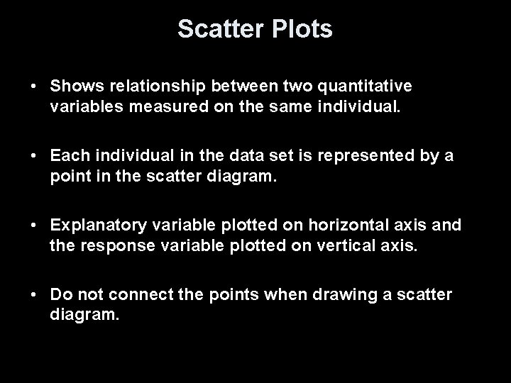
Scatter Plots • Shows relationship between two quantitative variables measured on the same individual. • Each individual in the data set is represented by a point in the scatter diagram. • Explanatory variable plotted on horizontal axis and the response variable plotted on vertical axis. • Do not connect the points when drawing a scatter diagram.

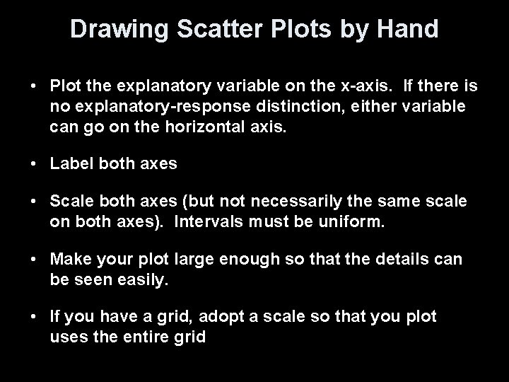
Drawing Scatter Plots by Hand • Plot the explanatory variable on the x-axis. If there is no explanatory-response distinction, either variable can go on the horizontal axis. • Label both axes • Scale both axes (but not necessarily the same scale on both axes). Intervals must be uniform. • Make your plot large enough so that the details can be seen easily. • If you have a grid, adopt a scale so that you plot uses the entire grid

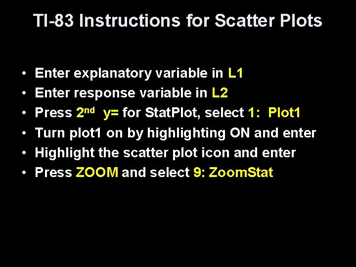
TI-83 Instructions for Scatter Plots • • • Enter explanatory variable in L 1 Enter response variable in L 2 Press 2 nd y= for Stat. Plot, select 1: Plot 1 Turn plot 1 on by highlighting ON and enter Highlight the scatter plot icon and enter Press ZOOM and select 9: Zoom. Stat

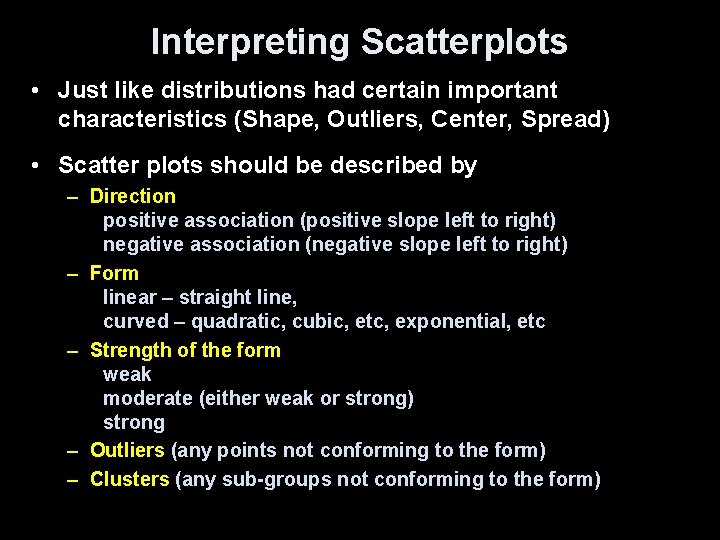
Interpreting Scatterplots • Just like distributions had certain important characteristics (Shape, Outliers, Center, Spread) • Scatter plots should be described by – Direction positive association (positive slope left to right) negative association (negative slope left to right) – Form linear – straight line, curved – quadratic, cubic, etc, exponential, etc – Strength of the form weak moderate (either weak or strong) strong – Outliers (any points not conforming to the form) – Clusters (any sub-groups not conforming to the form)

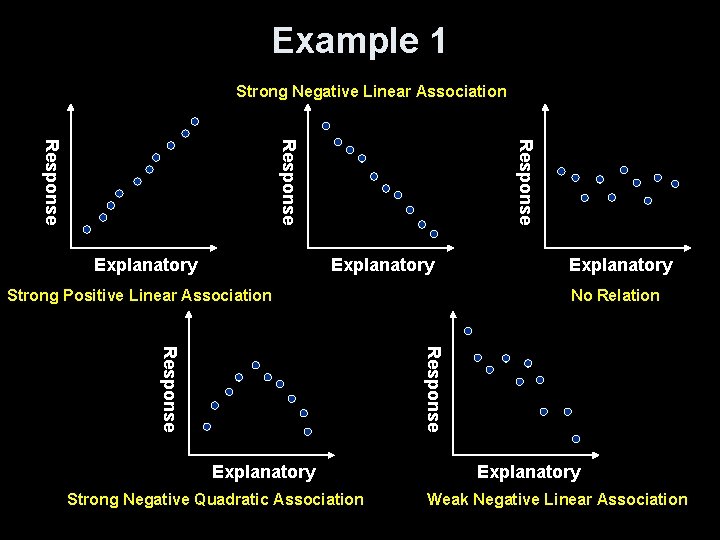
Example 1 Strong Negative Linear Association Response Explanatory Strong Positive Linear Association Explanatory No Relation Response Explanatory Strong Negative Quadratic Association Explanatory Weak Negative Linear Association

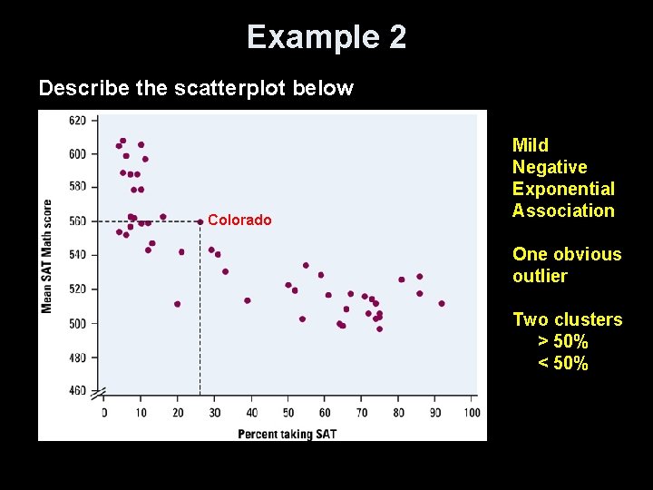
Example 2 Describe the scatterplot below Colorado Mild Negative Exponential Association One obvious outlier Two clusters > 50% < 50%

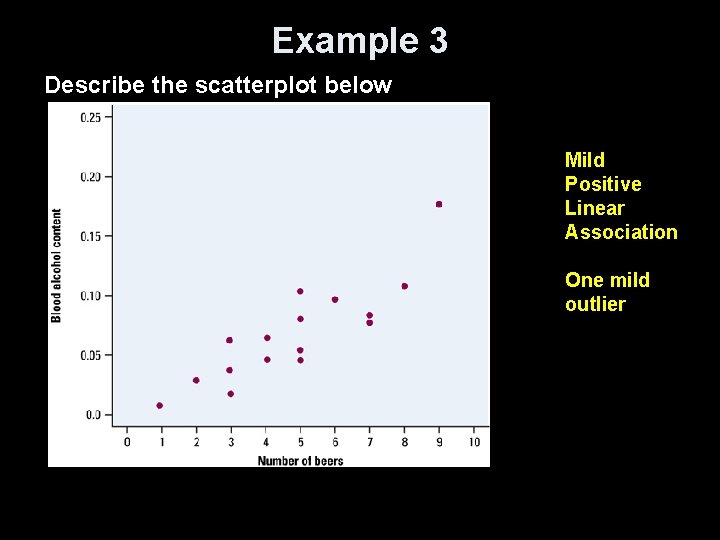
Example 3 Describe the scatterplot below Mild Positive Linear Association One mild outlier

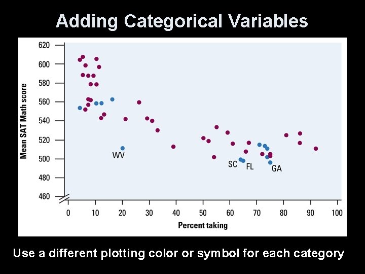
Adding Categorical Variables Use a different plotting color or symbol for each category

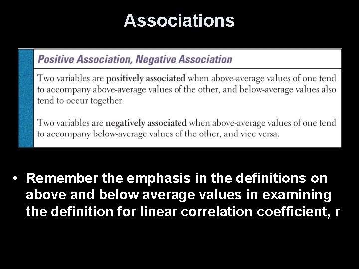
Associations • Remember the emphasis in the definitions on above and below average values in examining the definition for linear correlation coefficient, r

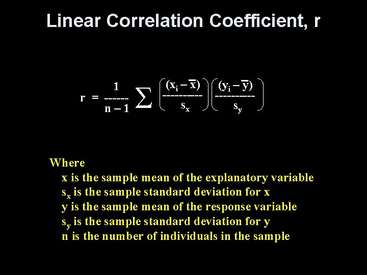
Linear Correlation Coefficient, r 1 r = -----n– 1 Σ (xi – x) (yi – y) -----sx sy Where x is the sample mean of the explanatory variable sx is the sample standard deviation for x y is the sample mean of the response variable sy is the sample standard deviation for y n is the number of individuals in the sample

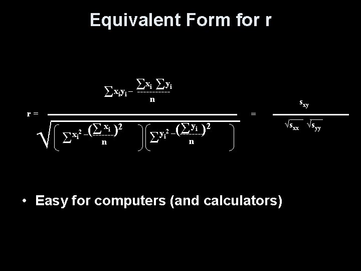
Equivalent Form for r Σ Σ Σ xi yi xiyi – -----n sxy r= √ = Σ xi 2 ( Σ – ----) n Σ yi 2 Σ yi )2 –(-------n • Easy for computers (and calculators) √sxx √syy

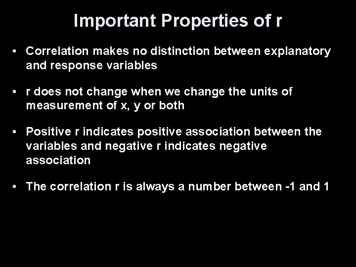
Important Properties of r • Correlation makes no distinction between explanatory and response variables • r does not change when we change the units of measurement of x, y or both • Positive r indicates positive association between the variables and negative r indicates negative association • The correlation r is always a number between -1 and 1

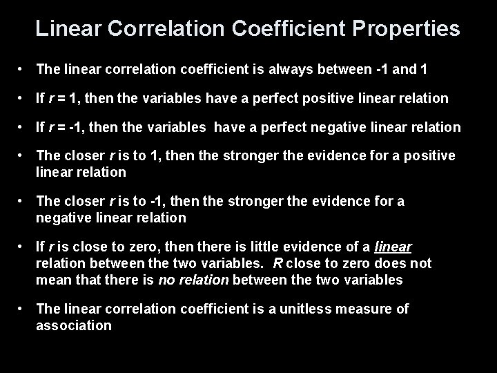
Linear Correlation Coefficient Properties • The linear correlation coefficient is always between -1 and 1 • If r = 1, then the variables have a perfect positive linear relation • If r = -1, then the variables have a perfect negative linear relation • The closer r is to 1, then the stronger the evidence for a positive linear relation • The closer r is to -1, then the stronger the evidence for a negative linear relation • If r is close to zero, then there is little evidence of a linear relation between the two variables. R close to zero does not mean that there is no relation between the two variables • The linear correlation coefficient is a unitless measure of association

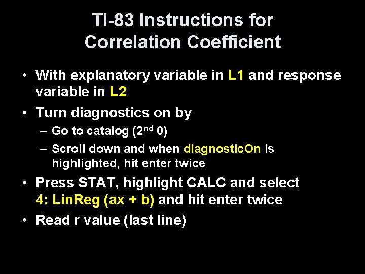
TI-83 Instructions for Correlation Coefficient • With explanatory variable in L 1 and response variable in L 2 • Turn diagnostics on by – Go to catalog (2 nd 0) – Scroll down and when diagnostic. On is highlighted, hit enter twice • Press STAT, highlight CALC and select 4: Lin. Reg (ax + b) and hit enter twice • Read r value (last line)

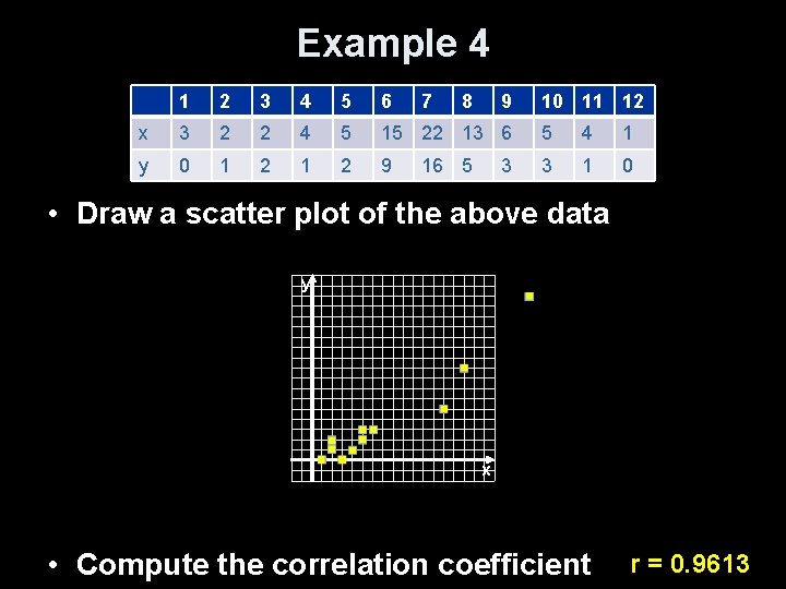
Example 4 1 2 3 4 5 6 7 8 9 x 3 2 2 4 5 15 22 13 6 5 4 1 y 0 1 2 9 3 1 0 16 5 3 10 11 12 • Draw a scatter plot of the above data y x • Compute the correlation coefficient r = 0. 9613

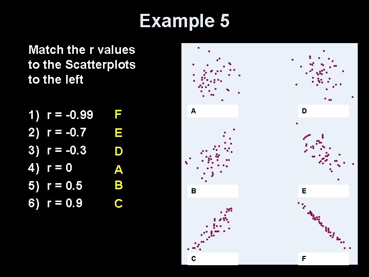
Example 5 Match the r values to the Scatterplots to the left 1) 2) 3) 4) 5) 6) r = -0. 99 r = -0. 7 r = -0. 3 r=0 r = 0. 5 r = 0. 9 F E D A B C A D B E C F

Cautions to Heed • Correlation requires that both variables be quantitative, so that it makes sense to do the arithmetic indicated by the formula for r • Correlation does not describe curved relationships between variables, not matter how strong they are • Like the mean and the standard deviation, the correlation is not resistant: r is strongly affected by a few outlying observations • Correlation is not a complete summary of two -variable data

Observational Data Reminder • If bivariate (two variable) data are observational, then we cannot conclude that any relation between the explanatory and response variable are due to cause and effect • Remember Observational versus Experimental Data

Summary and Homework • Summary – Scatter plots can show associations between variables and are described using direction, form, strength and outliers – Correlation r measures the strength and direction of the linear association between two variables – r ranges between -1 and 1 with 0 indicating no linear association • Homework – 3. 7, 3. 8, 3. 13 – 3. 16, 3. 21