Lesson 2 2 Organizing Quantitative Data The popular

Lesson 2 - 2 Organizing Quantitative Data: The popular displays

Objectives • Organize discrete data in tables • Construct histograms of discrete data • Organize continuous data in tables • Construct histograms of continuous data • Draw stem-and-leaf plots • Draw dot plots • Identify the shape of the distribution

Vocabulary • Histogram – bar graphs of the frequency or relative frequency of the class • Classes – categories of data • Lower class limit – smallest value in the class • Upper class limit – largest value in the class • Class width – largest value minus smallest value of the class • Open Ended – one of the limits is missing (or infinite) • Stem-and-Leaf Plot – numerical graph of the data organized by place of the digits • Split stems – divides the digit (range) in half • Dot plots – like a histogram, but with dots representing the bars • Data distribution – determining from the histogram the shape of the data

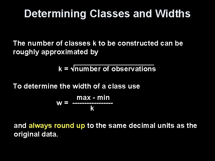
Determining Classes and Widths The number of classes k to be constructed can be roughly approximated by k = number of observations To determine the width of a class use max - min w = --------k and always round up to the same decimal units as the original data.

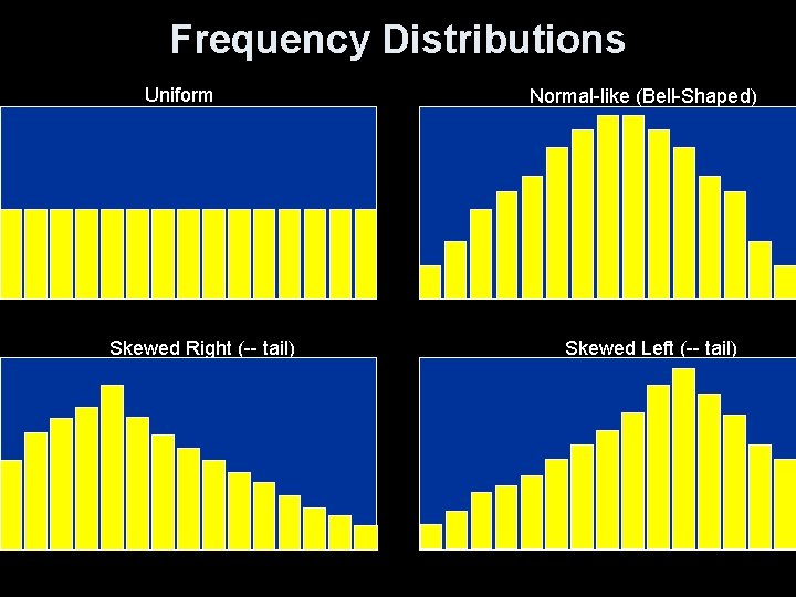
Frequency Distributions Uniform Skewed Right (-- tail) Normal-like (Bell-Shaped) Skewed Left (-- tail)

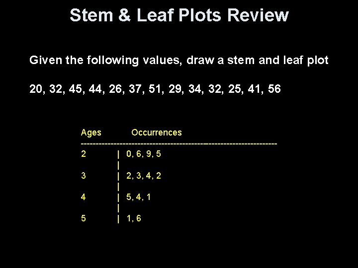
Stem & Leaf Plots Review Given the following values, draw a stem and leaf plot 20, 32, 45, 44, 26, 37, 51, 29, 34, 32, 25, 41, 56 Ages Occurrences ---------------------------------2 | 0, 6, 9, 5 | 3 | 2, 3, 4, 2 | 4 | 5, 4, 1 | 5 | 1, 6

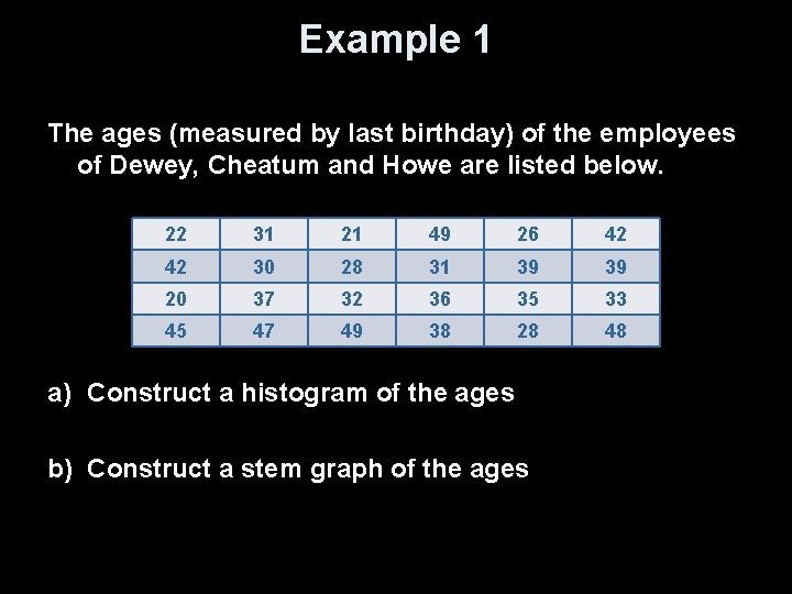
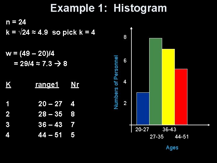
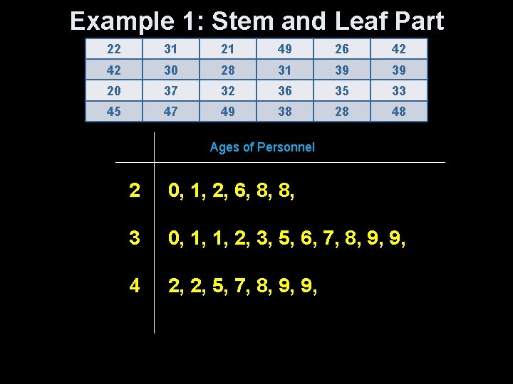
Example 1 The ages (measured by last birthday) of the employees of Dewey, Cheatum and Howe are listed below. 22 31 21 49 26 42 42 30 28 31 39 39 20 37 32 36 35 33 45 47 49 38 28 48 a) Construct a histogram of the ages b) Construct a stem graph of the ages

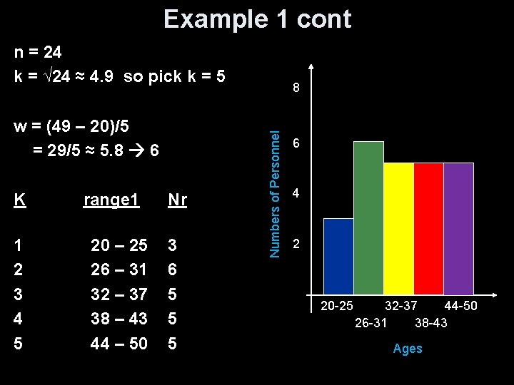
Example 1 cont n = 24 k = √ 24 ≈ 4. 9 so pick k = 5 K 1 2 3 4 5 range 1 20 – 25 26 – 31 32 – 37 38 – 43 44 – 50 Nr 3 6 5 5 5 Numbers of Personnel w = (49 – 20)/5 = 29/5 ≈ 5. 8 6 8 6 4 2 20 -25 32 -37 44 -50 26 -31 38 -43 Ages

Example 1 cont n = 24 k = √ 24 ≈ 4. 9 so pick k = 5 K 1 2 3 4 5 range 1 20 – 25 26 – 31 32 – 37 38 – 43 44 – 50 Nr 3 6 5 5 5 Numbers of Personnel w = (49 – 20)/5 = 29/5 ≈ 5. 8 6 8 6 4 2 20 26 32 38 Ages 44 50

Example 1: Histogram n = 24 k = √ 24 ≈ 4. 9 so pick k = 4 K 1 2 3 4 range 1 20 – 27 28 – 35 36 – 43 44 – 51 Nr 4 8 7 5 Numbers of Personnel w = (49 – 20)/4 = 29/4 ≈ 7. 3 8 8 6 4 2 20 -27 36 -43 27 -35 44 -51 Ages

Example 1: Stem and Leaf Part 22 31 21 49 26 42 42 30 28 31 39 39 20 37 32 36 35 33 45 47 49 38 28 48 Ages of Personnel 2 0, 1, 2, 6, 8, 8, 3 0, 1, 1, 2, 3, 5, 6, 7, 8, 9, 9, 4 2, 2, 5, 7, 8, 9, 9,

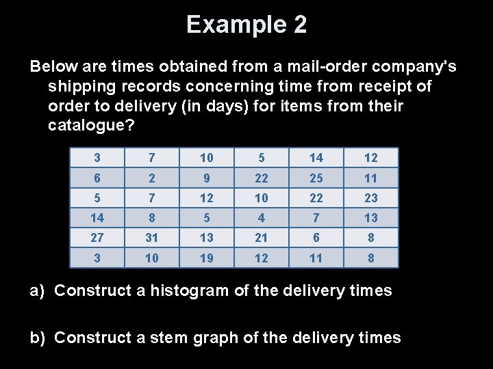
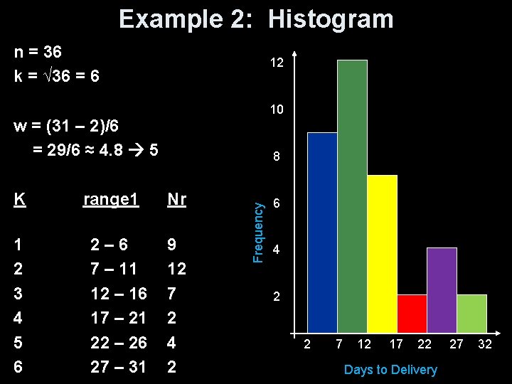
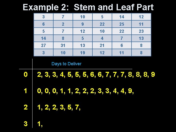
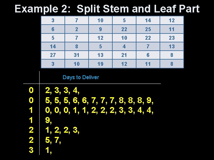
Example 2 Below are times obtained from a mail-order company's shipping records concerning time from receipt of order to delivery (in days) for items from their catalogue? 3 7 10 5 14 12 6 2 9 22 25 11 5 7 12 10 22 23 14 8 5 4 7 13 27 31 13 21 6 8 3 10 19 12 11 8 a) Construct a histogram of the delivery times b) Construct a stem graph of the delivery times

Example 2: Histogram n = 36 k = √ 36 = 6 12 10 w = (31 – 2)/6 = 29/6 ≈ 4. 8 5 1 2 3 4 5 6 range 1 2– 6 7 – 11 12 – 16 17 – 21 22 – 26 27 – 31 Nr 9 12 7 2 4 2 Frequency K 8 6 4 2 2 7 12 17 22 Days to Delivery 27 32

Example 2: Stem and Leaf Part 3 7 10 5 14 12 6 2 9 22 25 11 5 7 12 10 22 23 14 8 5 4 7 13 27 31 13 21 6 8 3 10 19 12 11 8 Days to Deliver 0 2, 3, 3, 4, 5, 5, 5, 6, 6, 7, 7, 7, 8, 8, 8, 9 1 0, 0, 0, 1, 1, 2, 2, 2, 3, 3, 4, 4, 9, 2 1, 2, 2, 3, 5, 7, 3 1,

Example 2: Split Stem and Leaf Part 3 7 10 5 14 12 6 2 9 22 25 11 5 7 12 10 22 23 14 8 5 4 7 13 27 31 13 21 6 8 3 10 19 12 11 8 Days to Deliver 0 0 1 1 2 2 3 2, 3, 3, 4, 5, 5, 5, 6, 6, 7, 7, 7, 8, 8, 8, 9, 0, 0, 0, 1, 1, 2, 2, 2, 3, 3, 4, 4, 9, 1, 2, 2, 3, 5, 7, 1,

Time Series Plot • Time on the x-axis • Interested values on the y-axis

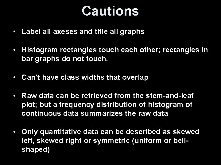
Cautions • Label all axeses and title all graphs • Histogram rectangles touch each other; rectangles in bar graphs do not touch. • Can’t have class widths that overlap • Raw data can be retrieved from the stem-and-leaf plot; but a frequency distribution of histogram of continuous data summarizes the raw data • Only quantitative data can be described as skewed left, skewed right or symmetric (uniform or bellshaped)

Summary and Homework • Summary – Stem & Leaf plots maintain the raw data, while histograms do not maintain the raw data – Best used when the data sets are small • Homework: – pg 87 - 96: 3, 6, 8, 9, 12, 14, 19, 28, 43