LESSON 17 AltitudeIntercept Method Learning Objectives Comprehend the

LESSON 17: Altitude-Intercept Method • Learning Objectives – Comprehend the concept of the circle of equal altitude as a line of position. – Become familiar with the concepts of the circle of equal altitude. – Know the altitude-intercept method of plotting a celestial LOP.

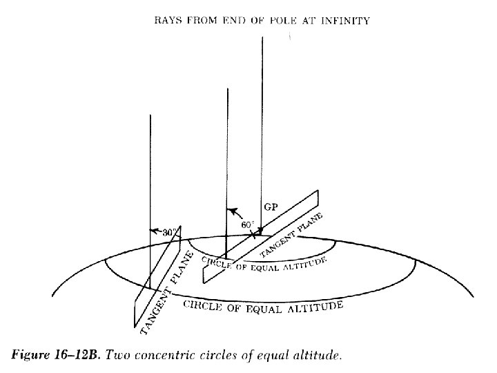
Circle of Equal Altitude • Imagine a pole attached to a flat surface, with a wire suspended from the pole. • If the wire is held at a constant angle to the pole, and rotated about the pole, it inscribes a circle. • This scenario is depicted on the next slide. . .

Circle of Equal Altitude • Now, let’s make two changes to our situation: – make the pole infinitely tall – make our surface spherical • Now we have something similar to the earth and the navigational stars. • Now our circles look like this. . .

Circle of Equal Altitude • Now, we need to relate this concept to the navigation triangle:

Circle of Equal Altitude • If we know the altitude of a star (as measured using a marine sextant), we can draw a “circle of equal altitude” of radius equal to the coaltitude (the distance between the GP of the star and our AP. )

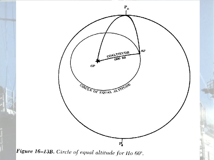
Circle of Equal Altitude • Thus, if we know the altitude of a particular star, and its location relative to the earth (which we can determine from the Nautical Almanac), we know that our position must lie somewhere on this circle of equal altitude. • Therefore, the circle of equal altitude is a line of position (LOP).

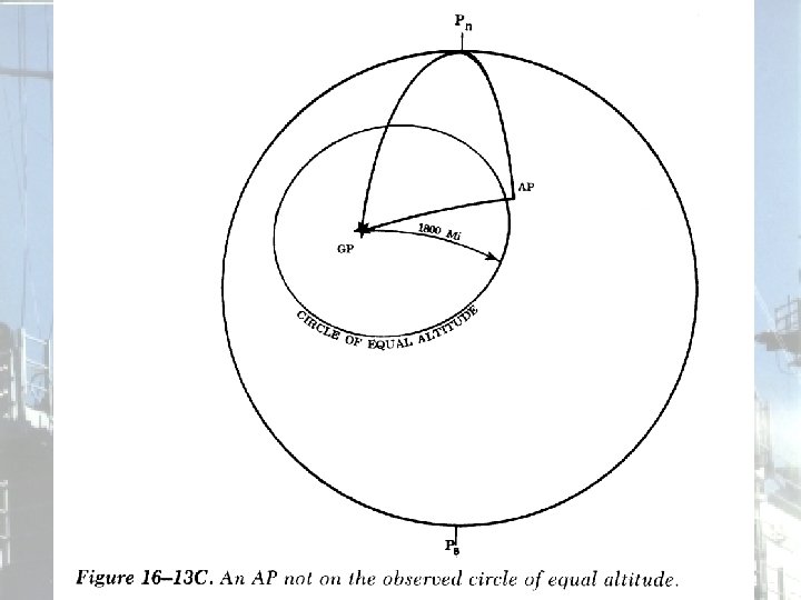
Circle of Equal Altitude • Here is a more realistic scenario, where our assumed position does not lie exactly on the circle of equal altitude. . .

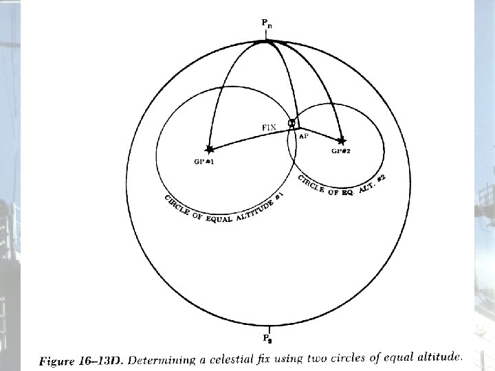
Circle of Equal Altitude • If we know the altitude of two or more stars, we can cross the LOP’s and arrive at a celestial fix. • Note that these circles cross at two points; however, these points are usually several hundred miles apart, and we can therefore rule one out. If not, a third star can be used to resolve the ambiguity.

Circle of Equal Altitude • Consider a problem with this idea: • For Ho=60 o, the radius of the circle of equal altitude is 1800 miles! To plot this with any degree of accuracy would require a chart larger than this room. • Instead, we only plot a small portion of this circle; this is the basis of the Altitude-Intercept Method.

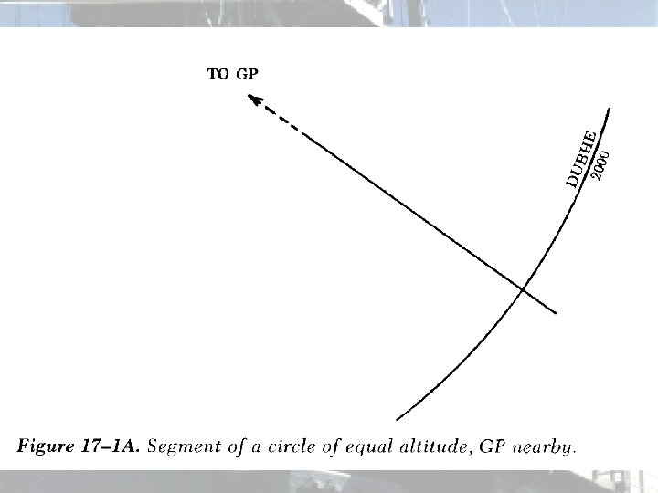
Altitude-Intercept Method • If we are near the GP, a portion of the circle would plot as an arc. . .

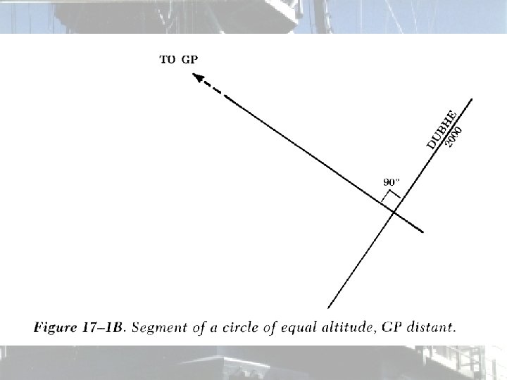
Altitude-Intercept Method • Now, if the distance to the GP is very large, the arc becomes a straight line. . .

Altitude-Intercept Method • Don’t forget, we are still essentially drawing a circle. • But we’re no longer using the radius (determined from the star’s altitude) so how do we know where, or for that matter, at what angle, to draw the line?

Altitude-Intercept Method • 1. First, assume a position based on the ship’s DR plot, and we modify the numbers slightly (for ease of calculation). • 2. Select navigational stars to shoot, and calculate what the altitude should be (Hc, computed altitude), given our AP and the time of observation.

Altitude-Intercept Method • 3. Observe the star’s altitude using a marine sextant, and determine the observed altitude (Ho). • 4. The difference between Hc and Ho, combined with Zn (which we can calculate using the Nautical Almanac and Pub 229) is used to plot a celestial LOP.

Altitude-Intercept Method • The difference between Hc and Ho is known as the intercept distance (a).

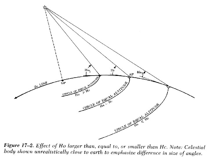
Altitude-Intercept Method • If Ho>Hc, we move toward the star (along Zn) to plot our celestial LOP. – “Ho Mo To” • If Hc>Ho, we move away from the star, along the reciprocal bearing of Zn, to plot our celestial LOP. – “Computed Greater Away” – “Coast Guard Academy”

Altitude-Intercept Method • A picture clearly illustrates the idea. . .

Example • Now let’s try an example to illustrate the concept: • A star is observed, and we determine that Ho is 45 o 00. 0’ • Based on our AP at the time of observation, Hc is 44 o 45. 5’

Example • First, we calculate the intercept distance, a, using a= Ho-Hc • The result is Ho -Hc a 45 o 00. 0’ 44 o 45. 5’ 14. 5’

Example • So our intercept distance is 14. 5 nm, and since Ho>Hc, we must move toward the star to plot our LOP. • Let’s examine again the angular relationships, and show the LOP is plotted. . .

Example

Plotting the Celestial LOP • Let’s assume we made an observation of Venus, and came up with – a = 14. 8 nm “towards” – Zn=091. 5 o T • The plotted LOP is shown on the next slide. . .

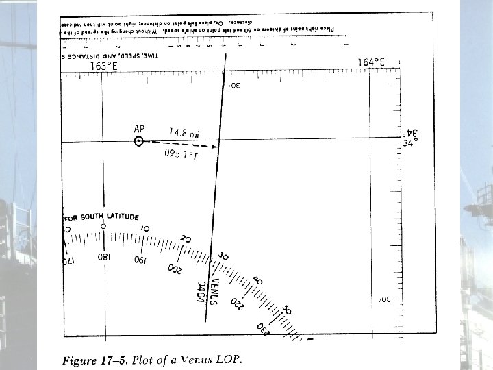
Plotting the Celestial LOP • Note that celestial plotting is usually done on a plotting sheet, and once a fix is established, the latitude and longitude are used to transfer it to the chart.