Lesson 16 Basic Control Modes ET 438 a

Lesson 16: Basic Control Modes ET 438 a Automatic Control Systems Technology lesson 16 et 438 a. pptx 1

Learning Objectives After this presentation you will be able to: Ø Ø Ø Describe the common control modes used in analog control systems List the characteristics of common control modes Write the time, Laplace and transfer functions of common control modes Identify the Bode plots of common control modes Design OP AMP circuits that realize theoretical control mode performance. lesson 16 et 438 a. pptx 2

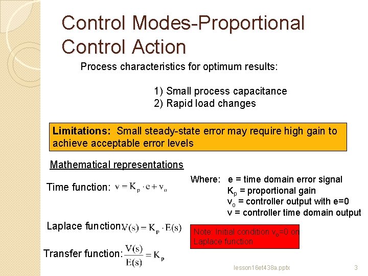
Control Modes-Proportional Control Action Process characteristics for optimum results: 1) Small process capacitance 2) Rapid load changes Limitations: Small steady-state error may require high gain to achieve acceptable error levels Mathematical representations Time function: Laplace function: Where: e = time domain error signal Kp = proportional gain vo = controller output with e=0 v = controller time domain output Note: Initial condition vo=0 on Laplace function Transfer function: lesson 16 et 438 a. pptx 3

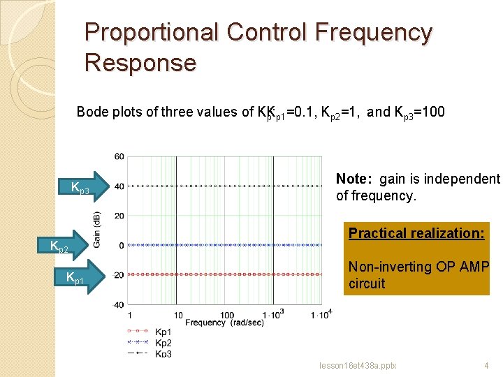
Proportional Control Frequency Response Bode plots of three values of KK p: p 1=0. 1, Kp 2=1, and Kp 3=100 Kp 3 Kp 2 Kp 1 Note: gain is independent of frequency. Practical realization: Non-inverting OP AMP circuit lesson 16 et 438 a. pptx 4

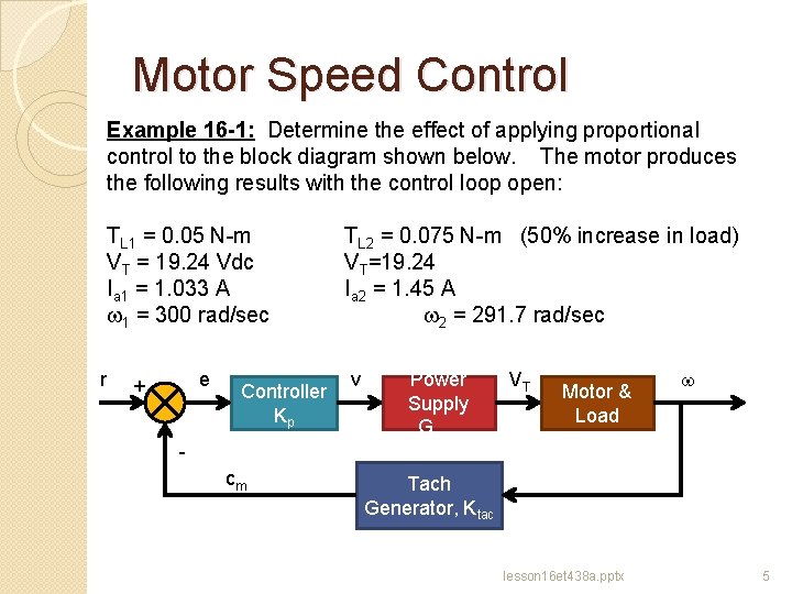
Motor Speed Control Example 16 -1: Determine the effect of applying proportional control to the block diagram shown below. The motor produces the following results with the control loop open: TL 1 = 0. 05 N-m VT = 19. 24 Vdc Ia 1 = 1. 033 A w 1 = 300 rad/sec r e + Controller Kp cm TL 2 = 0. 075 N-m (50% increase in load) VT=19. 24 Ia 2 = 1. 45 A w 2 = 291. 7 rad/sec v Power Supply Gamp VT Motor & Load w Tach Generator, Ktac lesson 16 et 438 a. pptx 5

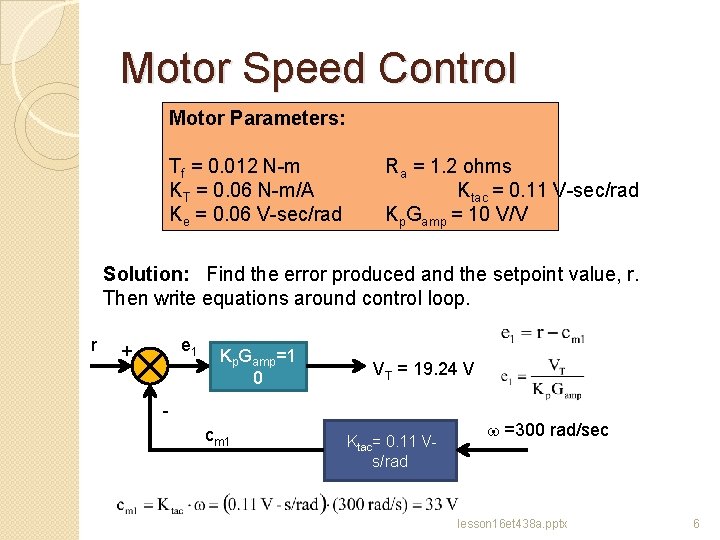
Motor Speed Control Motor Parameters: Tf = 0. 012 N-m KT = 0. 06 N-m/A Ke = 0. 06 V-sec/rad Ra = 1. 2 ohms Ktac = 0. 11 V-sec/rad Kp. Gamp = 10 V/V Solution: Find the error produced and the setpoint value, r. Then write equations around control loop. r e 1 + Kp. Gamp=1 0 VT = 19. 24 V cm 1 Ktac= 0. 11 Vs/rad w =300 rad/sec lesson 16 et 438 a. pptx 6

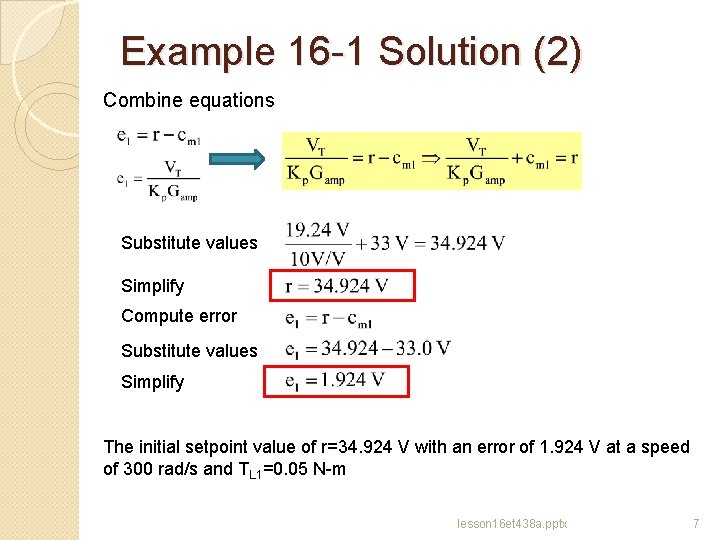
Example 16 -1 Solution (2) Combine equations Substitute values Simplify Compute error Substitute values Simplify The initial setpoint value of r=34. 924 V with an error of 1. 924 V at a speed of 300 rad/s and TL 1=0. 05 N-m lesson 16 et 438 a. pptx 7

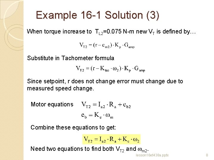
Example 16 -1 Solution (3) When torque increase to TL 2=0. 075 N-m new VT is defined by… Substitute in Tachometer formula Since setpoint, r does not change error must change due to measured speed change. Motor equations Combine these equations to get: Need two equations to find both VT 2 and wm 2. lesson 16 et 438 a. pptx 8

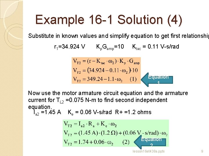
Example 16 -1 Solution (4) Substitute in known values and simplify equation to get first relationship r 1=34. 924 V Kp. Gamp=10 Ktac = 0. 11 V-s/rad Equation 1 Now use the motor armature circuit equation and the armature current for TL 2 =0. 075 N-m to find second independent equation. Ia 2 =1. 45 A Ke = 0. 06 V-s/rad R+ =1. 2 ohms Equation 2 lesson 16 et 438 a. pptx 9

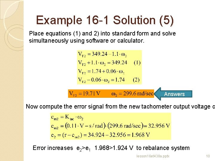
Example 16 -1 Solution (5) Place equations (1) and 2) into standard form and solve simultaneously using software or calculator. Answers Now compute the error signal from the new tachometer output voltage c Error increases e 2>e 1 1. 968>1. 924 V to rebalance system lesson 16 et 438 a. pptx 10

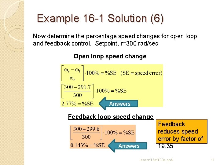
Example 16 -1 Solution (6) Now determine the percentage speed changes for open loop and feedback control. Setpoint, r=300 rad/sec Open loop speed change Answers Feedback reduces speed error by factor of 19. 35 lesson 16 et 438 a. pptx 11

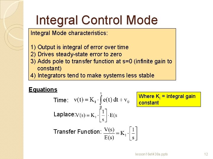
Integral Control Mode Integral Mode characteristics: 1) Output is integral of error over time 2) Drives steady-state error to zero 3) Adds pole to transfer function at s=0 (infinite gain to constant) 4) Integrators tend to make systems less stable Equations Time: Where KI = integral gain constant Laplace: Transfer Function: lesson 16 et 438 a. pptx 12

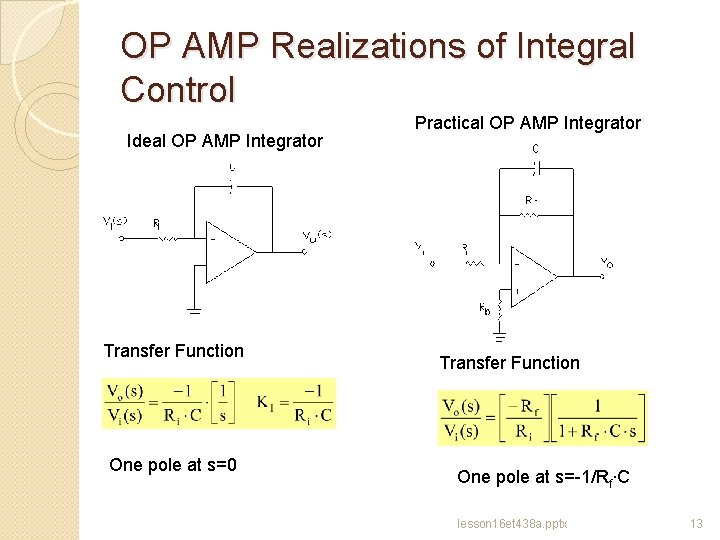
OP AMP Realizations of Integral Control Ideal OP AMP Integrator Transfer Function One pole at s=0 Practical OP AMP Integrator Transfer Function One pole at s=-1/Rf∙C lesson 16 et 438 a. pptx 13

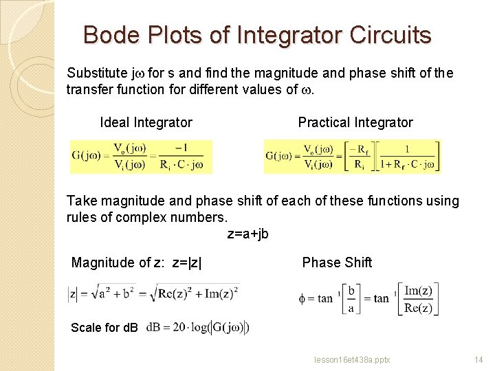
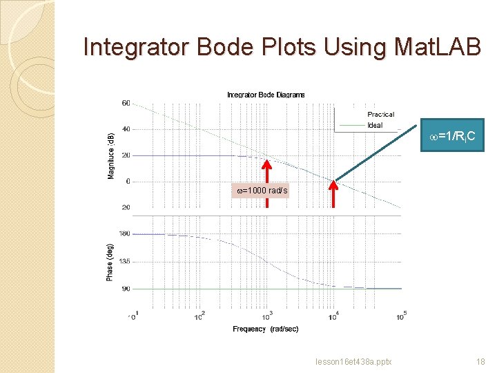
Bode Plots of Integrator Circuits Substitute jw for s and find the magnitude and phase shift of the transfer function for different values of w. Ideal Integrator Practical Integrator Take magnitude and phase shift of each of these functions using rules of complex numbers. z=a+jb Magnitude of z: z=|z| Phase Shift Scale for d. B lesson 16 et 438 a. pptx 14

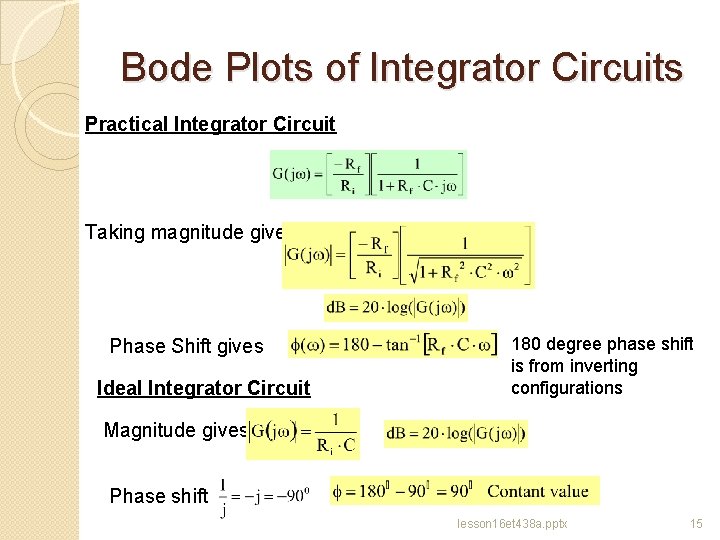
Bode Plots of Integrator Circuits Practical Integrator Circuit Taking magnitude gives Phase Shift gives Ideal Integrator Circuit 180 degree phase shift is from inverting configurations Magnitude gives Phase shift lesson 16 et 438 a. pptx 15

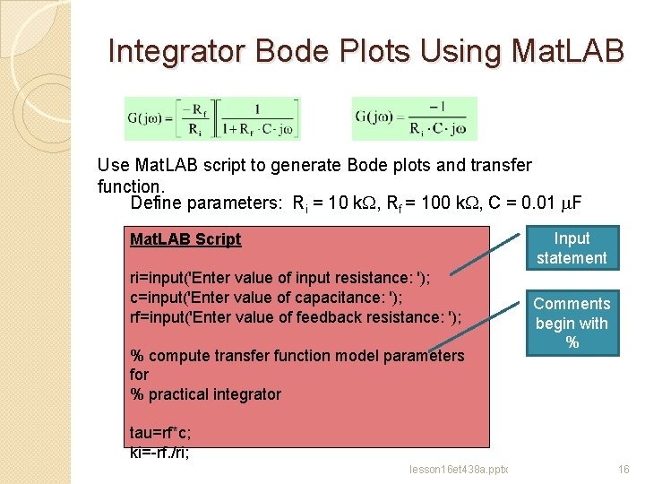
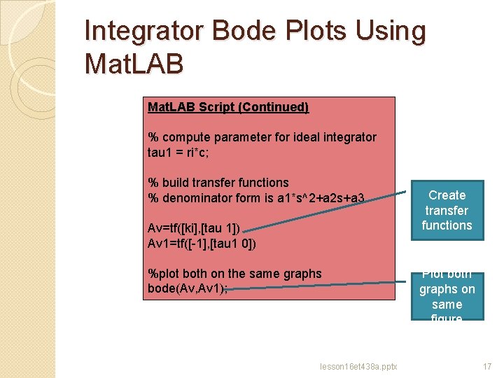
Integrator Bode Plots Using Mat. LAB Use Mat. LAB script to generate Bode plots and transfer function. Define parameters: Ri = 10 k. W, Rf = 100 k. W, C = 0. 01 m. F Input statement Mat. LAB Script ri=input('Enter value of input resistance: '); c=input('Enter value of capacitance: '); rf=input('Enter value of feedback resistance: '); % compute transfer function model parameters for % practical integrator Comments begin with % tau=rf*c; ki=-rf. /ri; lesson 16 et 438 a. pptx 16

Integrator Bode Plots Using Mat. LAB Script (Continued) % compute parameter for ideal integrator tau 1 = ri*c; % build transfer functions % denominator form is a 1*s^2+a 2 s+a 3 Av=tf([ki], [tau 1]) Av 1=tf([-1], [tau 1 0]) %plot both on the same graphs bode(Av, Av 1); lesson 16 et 438 a. pptx Create transfer functions Plot both graphs on same figure 17

Integrator Bode Plots Using Mat. LAB w=1/Ri. C w=1000 rad/s lesson 16 et 438 a. pptx 18

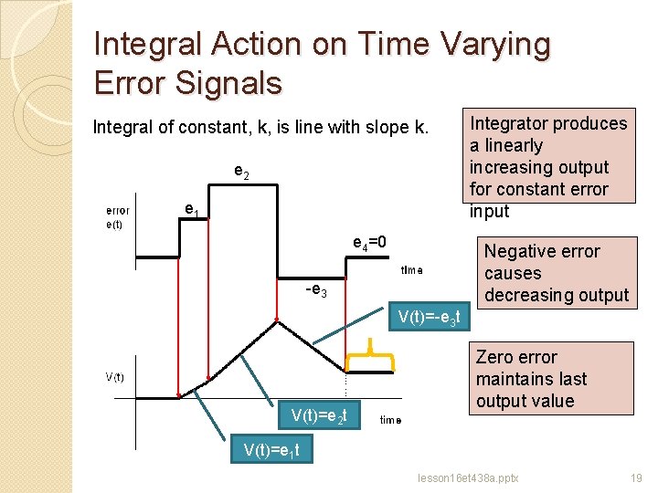
Integral Action on Time Varying Error Signals Integral of constant, k, is line with slope k. e 2 e 1 e 4=0 Integrator produces a linearly increasing output for constant error input Negative error causes decreasing output -e 3 V(t)=-e 3 t V(t)=e 2 t Zero error maintains last output value V(t)=e 1 t lesson 16 et 438 a. pptx 19

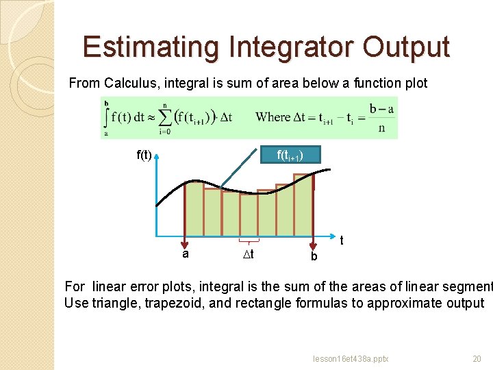
Estimating Integrator Output From Calculus, integral is sum of area below a function plot f(t) f(ti+1) a Dt t b For linear error plots, integral is the sum of the areas of linear segment Use triangle, trapezoid, and rectangle formulas to approximate output lesson 16 et 438 a. pptx 20

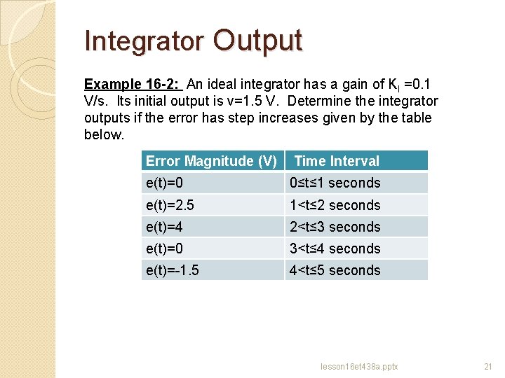
Integrator Output Example 16 -2: An ideal integrator has a gain of KI =0. 1 V/s. Its initial output is v=1. 5 V. Determine the integrator outputs if the error has step increases given by the table below. Error Magnitude (V) Time Interval e(t)=0 0≤t≤ 1 seconds e(t)=2. 5 1<t≤ 2 seconds e(t)=4 2<t≤ 3 seconds e(t)=0 3<t≤ 4 seconds e(t)=-1. 5 4<t≤ 5 seconds lesson 16 et 438 a. pptx 21

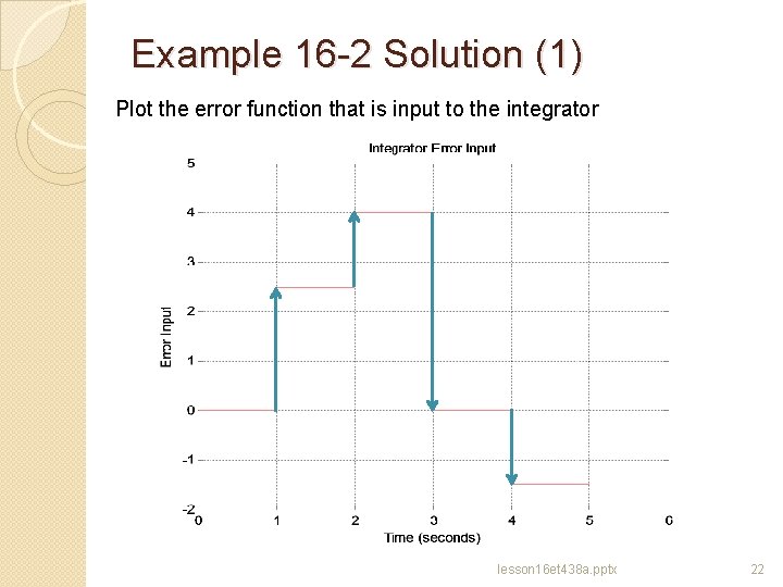
Example 16 -2 Solution (1) Plot the error function that is input to the integrator lesson 16 et 438 a. pptx 22

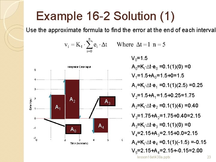
Example 16 -2 Solution (1) Use the approximate formula to find the error at the end of each interval V 0=1. 5 A 0=KI∙Dt∙e 0 =0. 1(1)(0) =0 V 1=1. 5+A 0=1. 5+0=1. 5 A 1=KI∙Dt∙e 1 =0. 1(1)(2. 5) =0. 25 A 2 A 3 A 1 V 2=1. 5+A 1=1. 5+0. 25=1. 75 A 2=KI∙Dt∙e 2 =0. 1(1)(4) =0. 40 V 3=1. 75+A 2=1. 75+0. 40=2. 15 A 0 A 4 A 3=KI∙Dt∙e 3 =0. 1(1)(0) =0 V 4=2. 15+A 3=2. 15+0. 0=2. 15 A 4=KI∙Dt∙e 4 =0. 1(1)(-1. 5) =-0. 15 V 5=2. 15+A 4=2. 15+-0. 15=2. 00 lesson 16 et 438 a. pptx 23

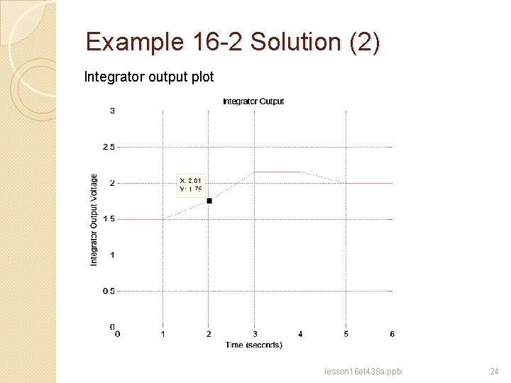
Example 16 -2 Solution (2) Integrator output plot lesson 16 et 438 a. pptx 24

Derivative Control Mode Derivative Control Characteristics: 1) Produces output only when error is changing 2) Output is proportional to rate of change in error 3) Derivative control never used alone 4) Used with proportional and/or integral modes 5) Anticipates error by observing the rate of change lesson 16 et 438 a. pptx 25

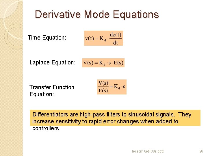
Derivative Mode Equations Time Equation: Laplace Equation: Transfer Function Equation: Differentiators are high-pass filters to sinusoidal signals. They increase sensitivity to rapid error changes when added to controllers. lesson 16 et 438 a. pptx 26

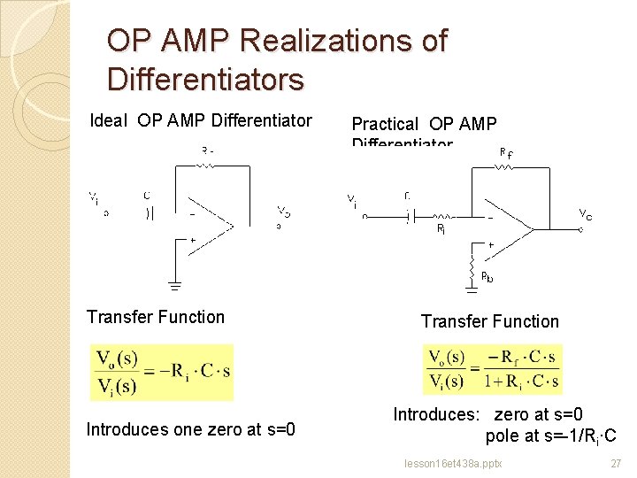
OP AMP Realizations of Differentiators Ideal OP AMP Differentiator Transfer Function Introduces one zero at s=0 Practical OP AMP Differentiator Transfer Function Introduces: zero at s=0 pole at s=-1/Ri∙C lesson 16 et 438 a. pptx 27

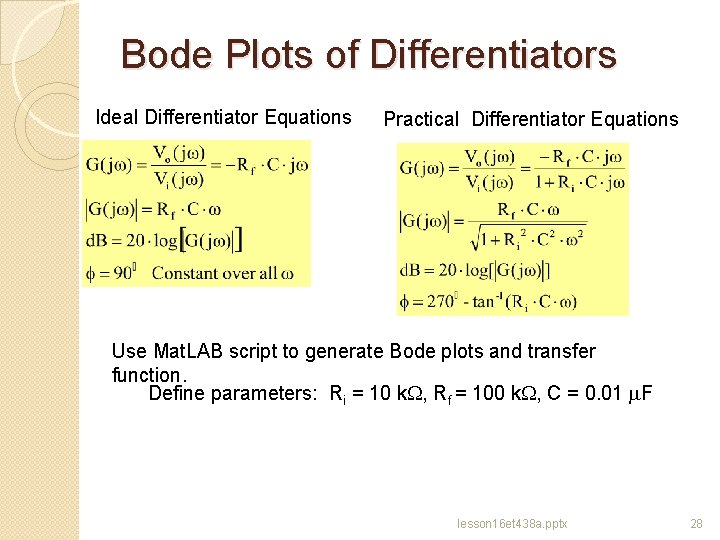
Bode Plots of Differentiators Ideal Differentiator Equations Practical Differentiator Equations Use Mat. LAB script to generate Bode plots and transfer function. Define parameters: Ri = 10 k. W, Rf = 100 k. W, C = 0. 01 m. F lesson 16 et 438 a. pptx 28

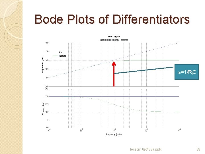
Bode Plots of Differentiators w=1/Ri. C lesson 16 et 438 a. pptx 29

ET 438 a Automatic Control Systems Technology END LESSON 16: BASIC CONTROL MODES lesson 16 et 438 a. pptx 30