Lesson 12 Creating Chart Activity 1 Activity 2

Lesson 12: Creating Chart

Activity 1: Activity 2: Student Achievement Chart Total Number Of Turtles Landing

Activity 1: Student Achievement Chart Activity 1. 1 Insert data in the worksheet 1. Open Microsoft Excel 2003 application. Type the data in the cells as shown below (Figure 1). Figure 1

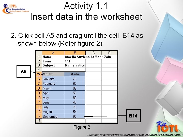
Activity 1. 1 Insert data in the worksheet 2. Click cell A 5 and drag until the cell B 14 as shown below (Refer figure 2) A 5 B 14 Figure 2

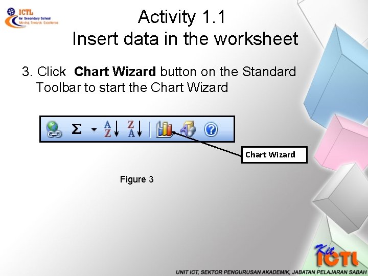
Activity 1. 1 Insert data in the worksheet 3. Click Chart Wizard button on the Standard Toolbar to start the Chart Wizard Figure 3

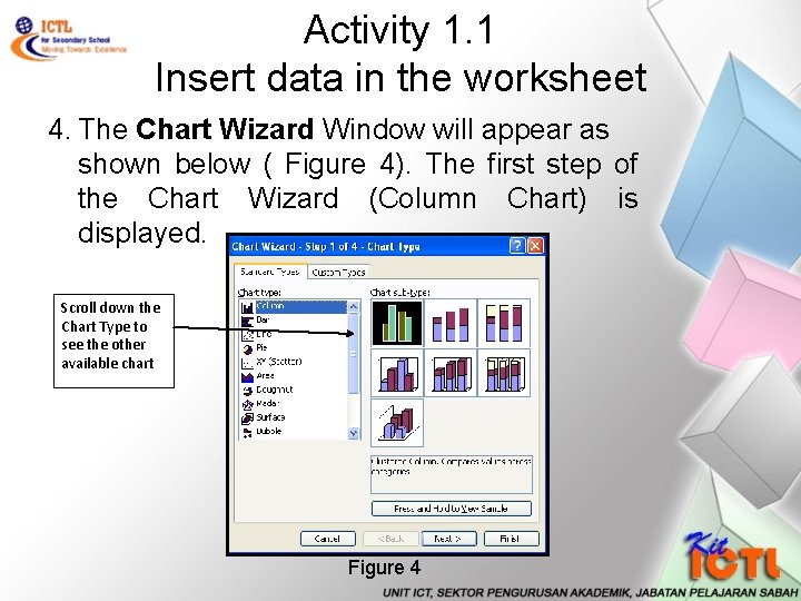
Activity 1. 1 Insert data in the worksheet 4. The Chart Wizard Window will appear as shown below ( Figure 4). The first step of the Chart Wizard (Column Chart) is displayed. Scroll down the Chart Type to see the other available chart Figure 4

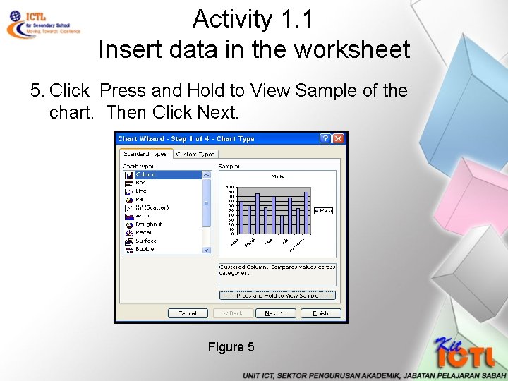
Activity 1. 1 Insert data in the worksheet 5. Click Press and Hold to View Sample of the chart. Then Click Next. Figure 5

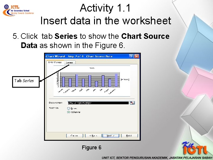
Activity 1. 1 Insert data in the worksheet 5. Click tab Series to show the Chart Source Data as shown in the Figure 6. Tab Series Figure 6

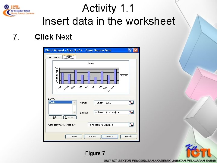
Activity 1. 1 Insert data in the worksheet 7. Click Next Figure 7

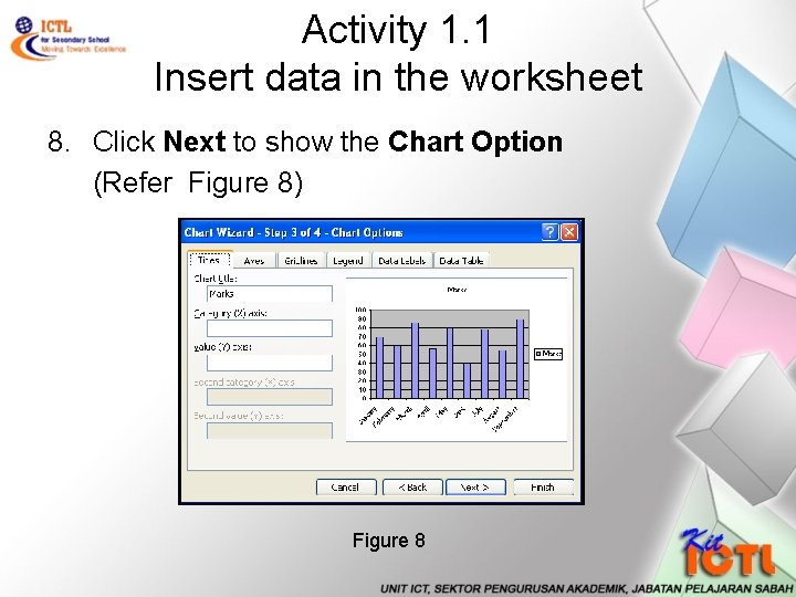
Activity 1. 1 Insert data in the worksheet 8. Click Next to show the Chart Option (Refer Figure 8) Figure 8

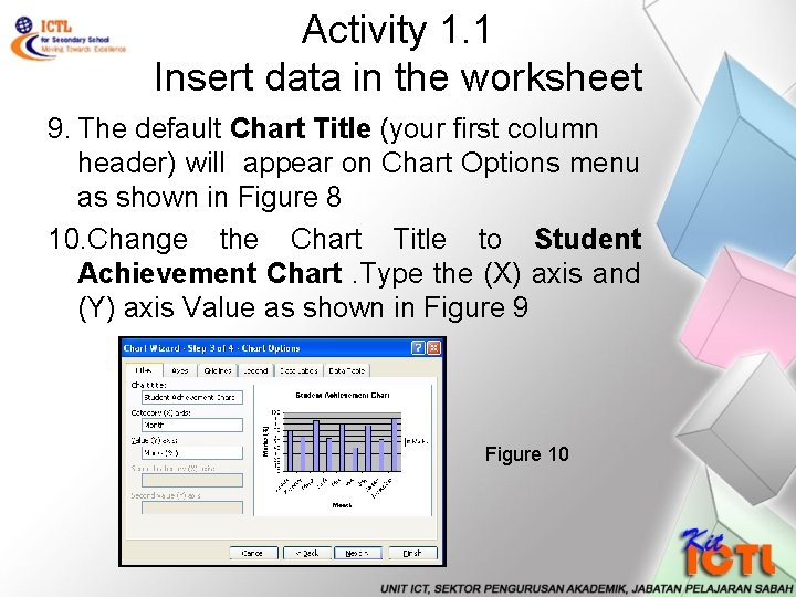
Activity 1. 1 Insert data in the worksheet 9. The default Chart Title (your first column header) will appear on Chart Options menu as shown in Figure 8 10. Change the Chart Title to Student Achievement Chart. Type the (X) axis and (Y) axis Value as shown in Figure 9 Figure 10

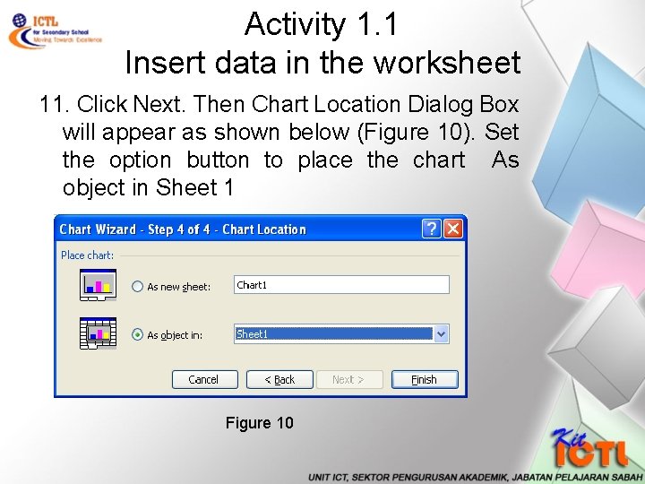
Activity 1. 1 Insert data in the worksheet 11. Click Next. Then Chart Location Dialog Box will appear as shown below (Figure 10). Set the option button to place the chart As object in Sheet 1 Figure 10

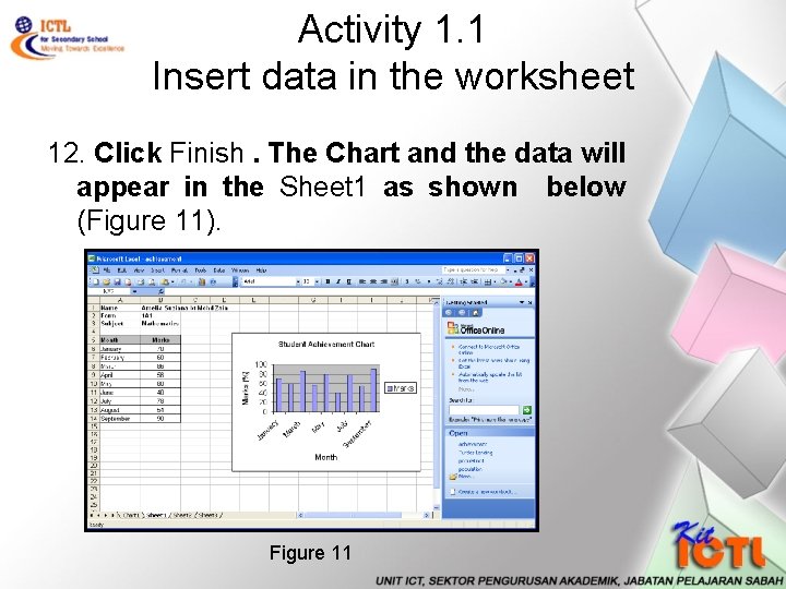
Activity 1. 1 Insert data in the worksheet 12. Click Finish. The Chart and the data will appear in the Sheet 1 as shown below (Figure 11). Figure 11

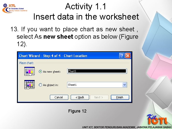
Activity 1. 1 Insert data in the worksheet 13. If you want to place chart as new sheet , select As new sheet option as below (Figure 12). Figure 12

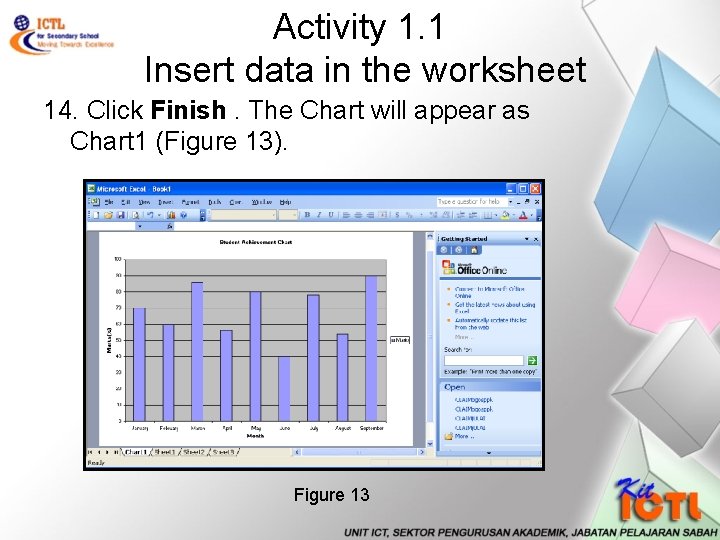
Activity 1. 1 Insert data in the worksheet 14. Click Finish. The Chart will appear as Chart 1 (Figure 13). Figure 13

Activity 1. 1 Insert data in the worksheet 15. Save your worksheet as achieve. xls in your on Folder. 16. To print the Chart, highlight the Chart. Then Click File, Print 17. Click OK. Then close your worksheet.

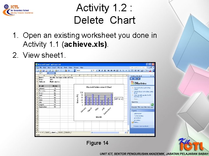
Activity 1. 2 : Delete Chart 1. Open an existing worksheet you done in Activity 1. 1 (achieve. xls). 2. View sheet 1. Figure 14

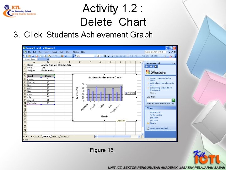
Activity 1. 2 : Delete Chart 3. Click Students Achievement Graph Figure 15

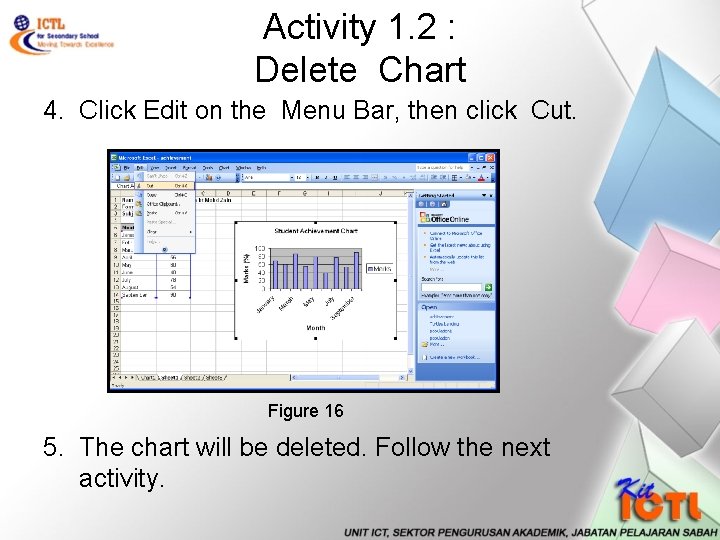
Activity 1. 2 : Delete Chart 4. Click Edit on the Menu Bar, then click Cut. Figure 16 5. The chart will be deleted. Follow the next activity.

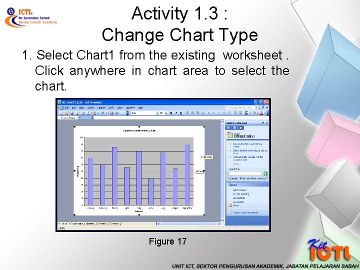
Activity 1. 3 : Change Chart Type 1. Select Chart 1 from the existing worksheet. Click anywhere in chart area to select the chart. Figure 17

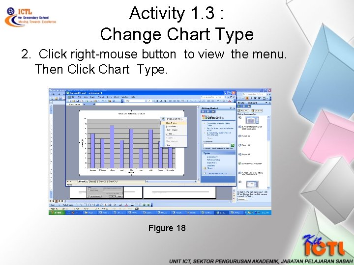
Activity 1. 3 : Change Chart Type 2. Click right-mouse button to view the menu. Then Click Chart Type. Figure 18

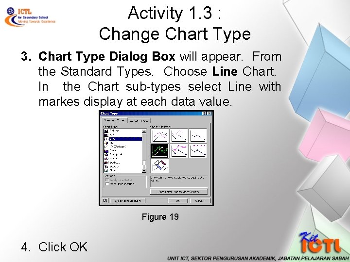
Activity 1. 3 : Change Chart Type 3. Chart Type Dialog Box will appear. From the Standard Types. Choose Line Chart. In the Chart sub-types select Line with markes display at each data value. Figure 19 4. Click OK

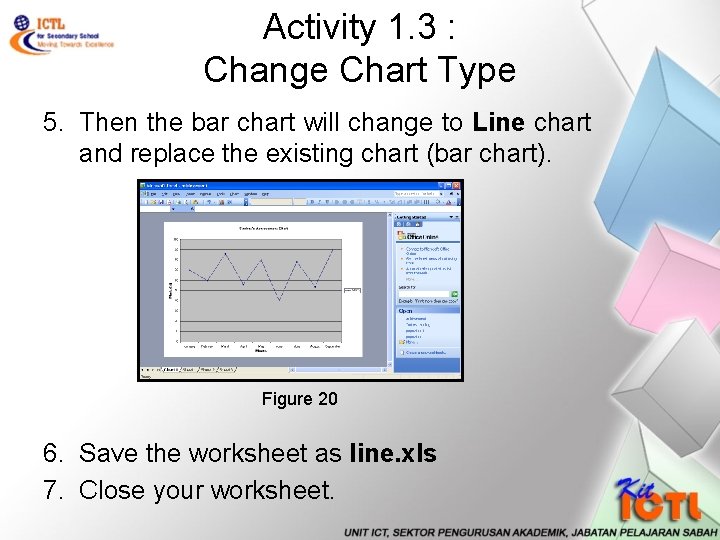
Activity 1. 3 : Change Chart Type 5. Then the bar chart will change to Line chart and replace the existing chart (bar chart). Figure 20 6. Save the worksheet as line. xls 7. Close your worksheet.

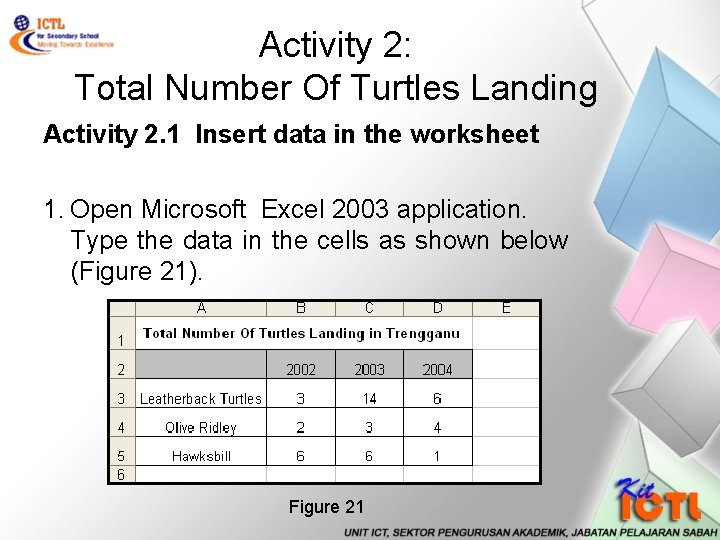
Activity 2: Total Number Of Turtles Landing Activity 2. 1 Insert data in the worksheet 1. Open Microsoft Excel 2003 application. Type the data in the cells as shown below (Figure 21). Figure 21

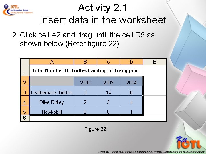
Activity 2. 1 Insert data in the worksheet 2. Click cell A 2 and drag until the cell D 5 as shown below (Refer figure 22) Figure 22

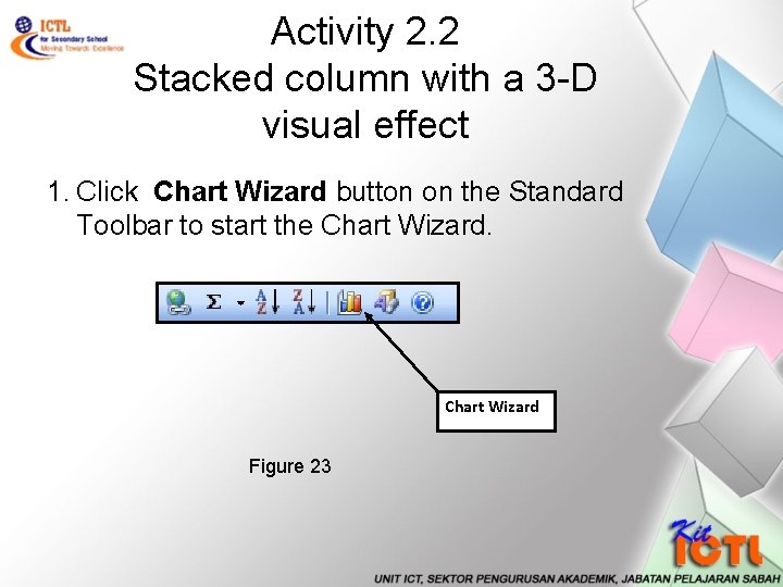
Activity 2. 2 Stacked column with a 3 -D visual effect 1. Click Chart Wizard button on the Standard Toolbar to start the Chart Wizard Figure 23

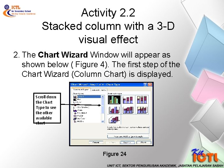
Activity 2. 2 Stacked column with a 3 -D visual effect 2. The Chart Wizard Window will appear as shown below ( Figure 4). The first step of the Chart Wizard (Column Chart) is displayed. Scroll down the Chart Type to see the other available chart Figure 24

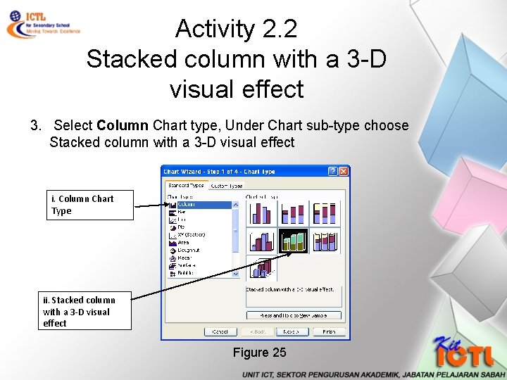
Activity 2. 2 Stacked column with a 3 -D visual effect 3. Select Column Chart type, Under Chart sub-type choose Stacked column with a 3 -D visual effect i. Column Chart Type ii. Stacked column with a 3 -D visual effect Figure 25

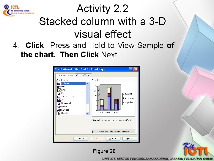
Activity 2. 2 Stacked column with a 3 -D visual effect 4. Click Press and Hold to View Sample of the chart. Then Click Next. Figure 26

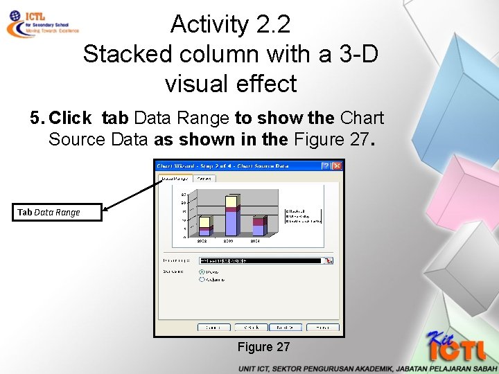
Activity 2. 2 Stacked column with a 3 -D visual effect 5. Click tab Data Range to show the Chart Source Data as shown in the Figure 27. Tab Data Range Figure 27

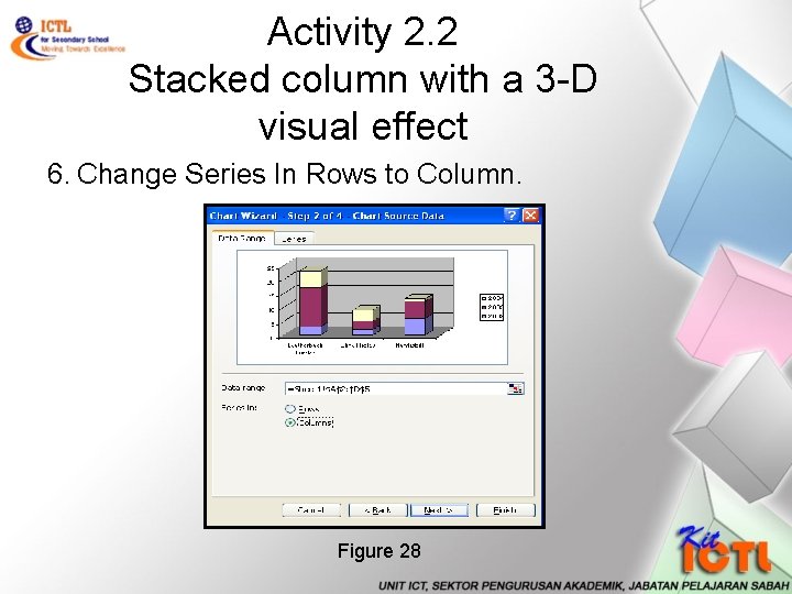
Activity 2. 2 Stacked column with a 3 -D visual effect 6. Change Series In Rows to Column. Figure 28

Activity 2. 2 Stacked column with a 3 -D visual effect 7. Click Next to show the Chart Options. Type Chart Title as Total Number of Turtle Landings in Terengganu , Categoy (X) axis as Turtles Type and Value (Z) axis as Number ( Figure 29) Figure 29

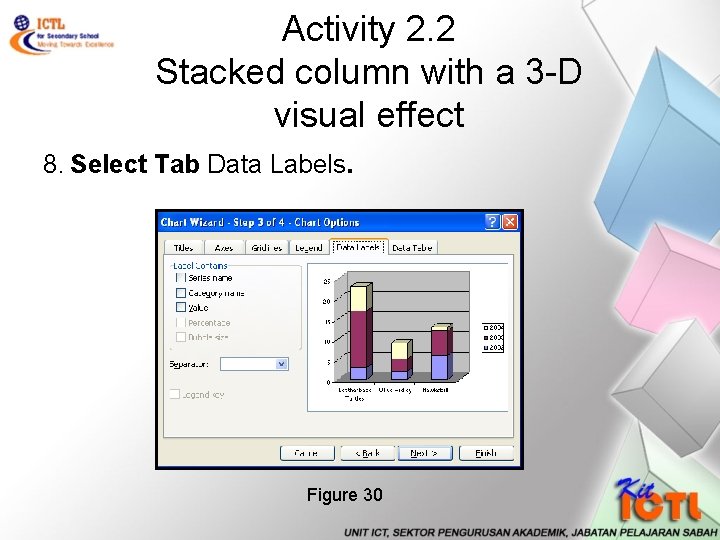
Activity 2. 2 Stacked column with a 3 -D visual effect 8. Select Tab Data Labels. Figure 30

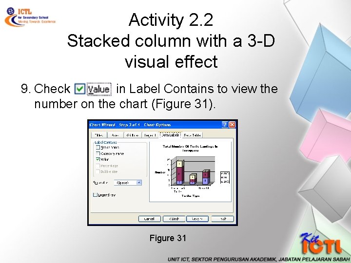
Activity 2. 2 Stacked column with a 3 -D visual effect 9. Check in Label Contains to view the number on the chart (Figure 31). Figure 31

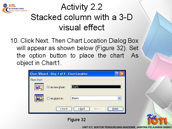
Activity 2. 2 Stacked column with a 3 -D visual effect 10. Click Next. Then Chart Location Dialog Box will appear as shown below (Figure 32). Set the option button to place the chart As object in Chart 1. Figure 32

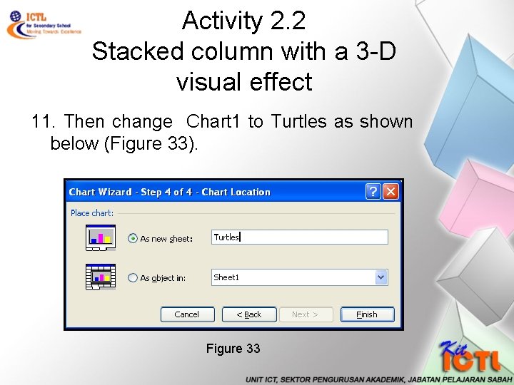
Activity 2. 2 Stacked column with a 3 -D visual effect 11. Then change Chart 1 to Turtles as shown below (Figure 33). Figure 33

Activity 2. 2 Stacked column with a 3 -D visual effect 12. Click Finish. The Chart will appear as Turtles (Figure 34). Figure 34

Activity 2. 2 Stacked column with a 3 -D visual effect 13. Save your worksheet as turtles. xls in your own Folder. 14. To print the Chart, highlight the Chart. Then Click File, Print 15. Click OK. Then close your worksheet.

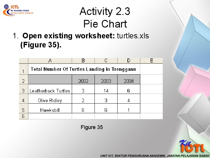
Activity 2. 3 Pie Chart 1. Open existing worksheet: turtles. xls (Figure 35). Figure 35

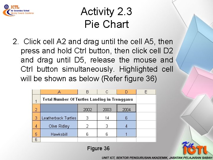
Activity 2. 3 Pie Chart 2. Click cell A 2 and drag until the cell A 5, then press and hold Ctrl button, then click cell D 2 and drag until D 5, release the mouse and Ctrl button simultaneously. Highlighted cell will be shown as below (Refer figure 36) Figure 36

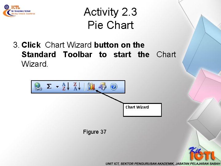
Activity 2. 3 Pie Chart 3. Click Chart Wizard button on the Standard Toolbar to start the Chart Wizard Figure 37

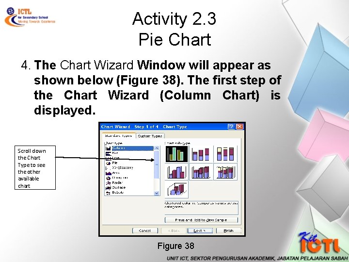
Activity 2. 3 Pie Chart 4. The Chart Wizard Window will appear as shown below (Figure 38). The first step of the Chart Wizard (Column Chart) is displayed. Scroll down the Chart Type to see the other available chart Figure 38

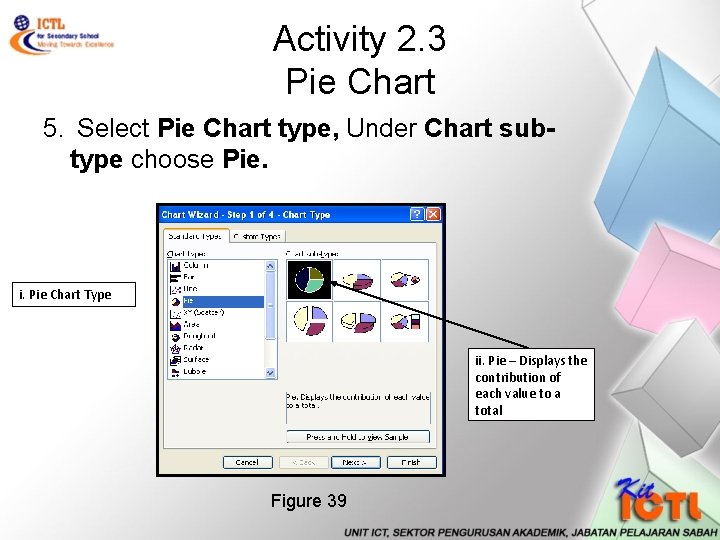
Activity 2. 3 Pie Chart 5. Select Pie Chart type, Under Chart subtype choose Pie. i. Pie Chart Type ii. Pie – Displays the contribution of each value to a total Figure 39

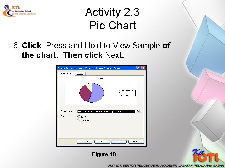
Activity 2. 3 Pie Chart 6. Click Press and Hold to View Sample of the chart. Then click Next. Figure 40

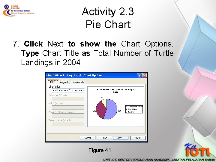
Activity 2. 3 Pie Chart 7. Click Next to show the Chart Options. Type Chart Title as Total Number of Turtle Landings in 2004 Figure 41

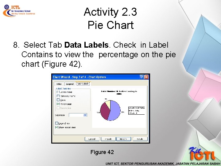
Activity 2. 3 Pie Chart 8. Select Tab Data Labels. Check in Label Contains to view the percentage on the pie chart (Figure 42). Figure 42

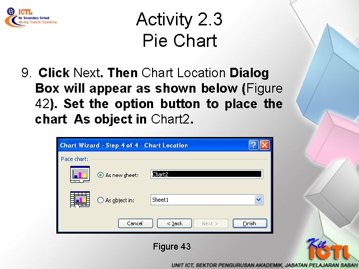
Activity 2. 3 Pie Chart 9. Click Next. Then Chart Location Dialog Box will appear as shown below (Figure 42). Set the option button to place the chart As object in Chart 2. Figure 43

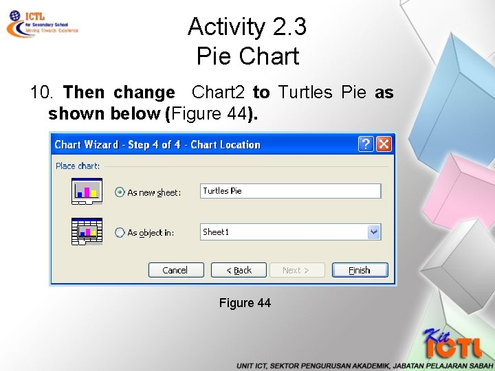
Activity 2. 3 Pie Chart 10. Then change Chart 2 to Turtles Pie as shown below (Figure 44). Figure 44

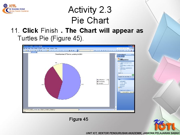
Activity 2. 3 Pie Chart 11. Click Finish. The Chart will appear as Turtles Pie (Figure 45). Figure 45

Activity 2. 3 Pie Chart 12. Save your worksheet. 13. To print the Chart, highlight the Chart. Then Click File, Print 14. Click OK. Then close your worksheet.