Leontief Paradox 1953 HO predicts that Kabundant USA

Leontief Paradox (1953) • HO predicts that K-abundant USA will – Export K-int products and import L-int products – Thus K/L ratio in exports >> K/L ratio in imports • Leontief found that – K/L ratio in exports << K/L ratio in imports

Leontief Paradox • Using 1947 US data and • Using his invention input-output tables • Assuming exports decrease by 1 million dollars leads to release of K and L >>> calculate K/L ratio in exports • Assuming imports decrease by 1 million dollar leads to reproduce by K and L >>> calculate K/L ratio in imports

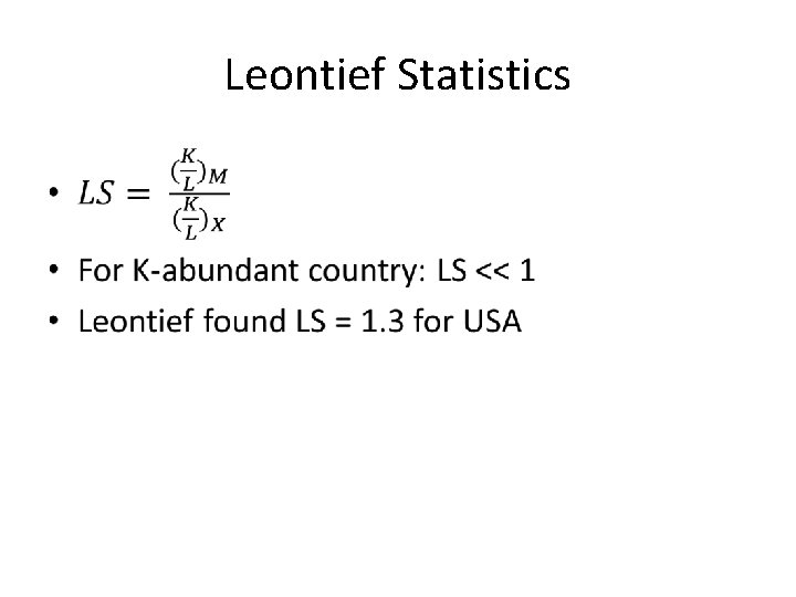
Leontief Statistics •

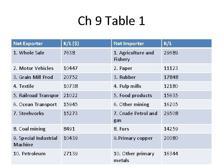
Ch 9 Table 1 Net Exporter K/L ($) Net Importer K/L 1. Whole Sale 7638 1. Agriculture and Fishery 29689 2. Motor Vehicles 10447 2. Paper 11123 3. Grain Mill Prod 20752 3. Rubber 17848 4. Textile 10738 4. Pulp mills 12180 5. Railroad Transpor 21022 5. Food products 15635 6. Ocean Transport 15945 6. Other mining 16205 7. Steelworks 15273 7. Crude Petrol and gas 29508 8. Coal mining 8491 8. Furs 14259 9. Special Industrial Machine 10439 9. Primary copper 20080 10. Petroleum 27139 10. Other primary metals 16344

Ch 9 Table 1 • • Out of 167 industrial sectors 10 largest net exporters 10 largest net importers for USA 7 out of 10 net importer sectors had higher K/L ratio than net exporter sectors

Explanations for Leontief Paradox • • • 1. Demand Factor 2. Factor Intensity Reversal 3. US Tariff Structure 4. Disaggregated Labor 5. Natural Resources

1. Demand Factor For example: If US consumers like K-int Steel too much and If US consumers like L-int Cloth too little Then price of steel may be high relative to price of cloth • Reversing HO-based comparative advantage • •

2. Factor Intensity Reversal • If goods are produced K-intensively in one country, and L-intensively in the other country. • Then HO-based Trade pattern does not happen. • Minhas (1962) – Used 1947 and 1951 US and Japan data – For 20 industries – Calculate K/L ratio in each sector

Minhas (1962) • Rank 20 industries according to K/L ratio in USA and in Japan • RANK CORRELATION is calculated between US and Japan • RC = 1 (the same order) • RC = -1 (the opposite order) • RC = 0 ( no relationship between the rank in USA and rank in Japan)

Minhas (1962) • Minhas found RC = 0. 328 • Low relationship between the ranks in US and Japan • Evidence against HO assumption of “No Factor -Intensity Reversal”

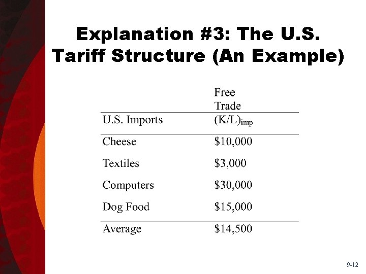
3. US Tariff Structure • • • HO states that abundant factor gains and scarce factor loses from trade In USA, Kapital gains; Labor loses Thus Labor is protectionist Thus more tariffs on L-int products EXAMPLE (below): Textile L-int, protected, became non-traded.

Explanation #3: The U. S. Tariff Structure (An Example) 9 -12

Explanation #3: The U. S. Tariff Structure (An Example) 9 -13

Explanation #3: The U. S. Tariff Structure (An Example) • Suppose that (K/L)exp = $16, 000. • Then the fact that tariffs exist means that the Leontief statistic is $18, 333/$16, 000 = 1. 14; it would have been $14, 500/$16, 000 = 0. 9 under the assumption of free trade. • This means that Leontief’s paradox might be the result of tariffs, and isn’t evidence against the H-O model.

3. US Tariff Structure • • • Baldwin (1971) show that (K/L)imp under tariffs is 5% less than (K/L)imp under free-trade Nevertheless his Leontief Stat LS > 1 Still US imports are more K-int than US exports.

4. Disaggregated Labor • • Keesing (1966) used disaggregated labor: (8 categories of labor): i. scientists and engineers ii. Technicians … viii. Unskilled labor Found: US exports had more of Category 1 US imports had more of Category 8.

5. Natural Resources • • Hartigan (1981) Calculated LS for 1947 and 1951 US data Paradox still exist (LS >> 1 for USA) But when he deletes NR industries, he finds: LS = 0. 917 for 1947 and LS = 0. 88 for 1951. Conclusion: US imports more of NR-int rather than K-int

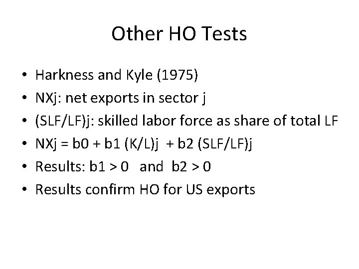
Other HO Tests • • • Harkness and Kyle (1975) NXj: net exports in sector j (SLF/LF)j: skilled labor force as share of total LF NXj = b 0 + b 1 (K/L)j + b 2 (SLF/LF)j Results: b 1 > 0 and b 2 > 0 Results confirm HO for US exports

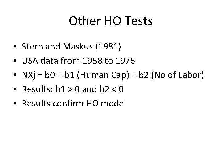
Other HO Tests • • • Stern and Maskus (1981) USA data from 1958 to 1976 NXj = b 0 + b 1 (Human Cap) + b 2 (No of Labor) Results: b 1 > 0 and b 2 < 0 Results confirm HO model

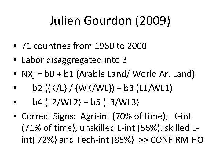
Julien Gourdon (2009) • • • 71 countries from 1960 to 2000 Labor disaggregated into 3 NXj = b 0 + b 1 (Arable Land/ World Ar. Land) b 2 ({K/L} / {WK/WL}) + b 3 (L 1/WL 1) b 4 (L 2/WL 2) + b 5 (L 3/WL 3) Correct Signs: Agri-int (70% of time); K-int (71% of time); unskilled L-int (56%); skilled Lint( 72%) and Tech-int (85%) >> CONFIRM HO

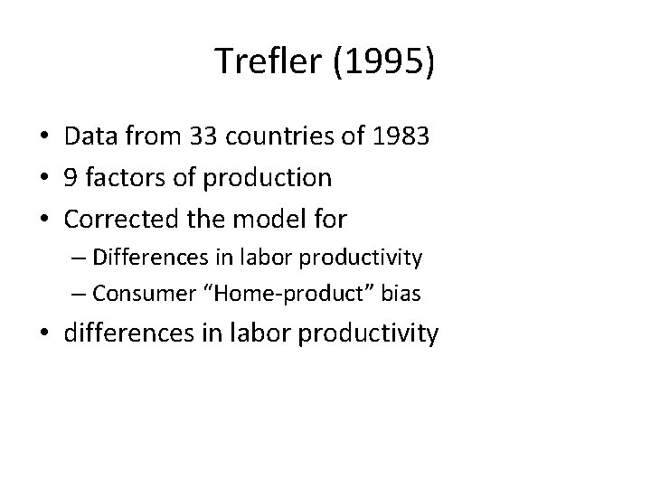
Trefler (1995) • Data from 33 countries of 1983 • 9 factors of production • Corrected the model for – Differences in labor productivity – Consumer “Home-product” bias • differences in labor productivity

HO-Vanek Model • Factor Content Approach • Production bundle gives “factors needed to produce” • Consumption bundle gives “ demand for each factor” • For any factor: if total production requirement is bigger than total consumption requirement • Then Country is exporting SERVICES of that factor

HO-Vanek Model • For any factor: if total production requirement is less than total consumption requirement • Then Country is importing SERVICES of that factor. • Thus K-abundant country will export Capital Services. • EX: Maskus(1985) uses 5 factors: engineers; production workers; nonproduction workers; physical capital; human capital. CONFIRM HO.

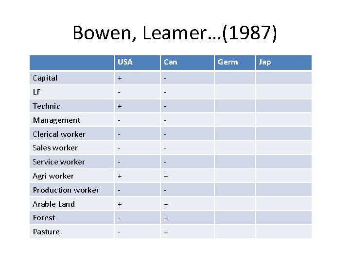
Bowen, Leamer…(1987) USA Can Capital + - LF - - Technic + - Management - - Clerical worker - - Sales worker - - Service worker - - Agri worker + + Production worker - - Arable Land + + Forest - + Pasture - + Germ Jap

Bowen, Leamer…(1987) • 27 countries; 12 Factors • Net exports (+); Net imports (-) • For example: USA is a net exporter of SERVICES of Agriculture workers. • Thus USA is REVEALED to be abundant in Agri workers.

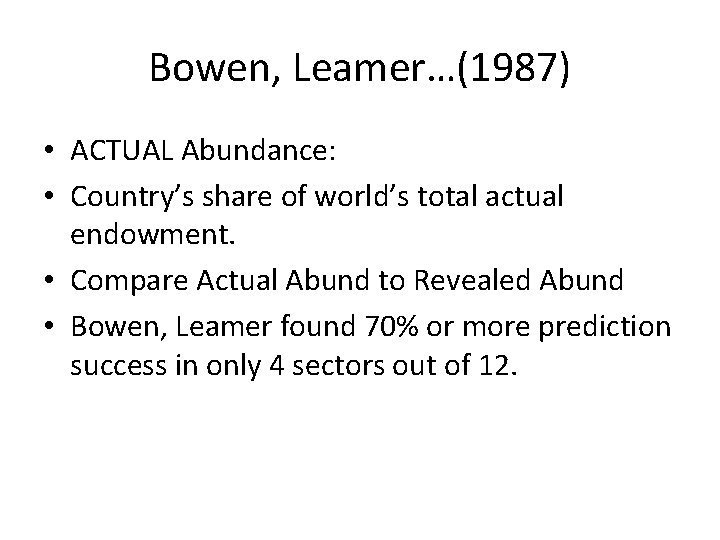
Bowen, Leamer…(1987) • ACTUAL Abundance: • Country’s share of world’s total actual endowment. • Compare Actual Abund to Revealed Abund • Bowen, Leamer found 70% or more prediction success in only 4 sectors out of 12.

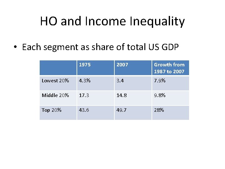
HO and Income Inequality • Each segment as share of total US GDP 1975 2007 Growth from 1987 to 2007 Lowest 20% 4. 3% 3. 4 7. 9% Middle 20% 17. 3 14. 8 9. 8% Top 20% 43. 6 49. 7 28%

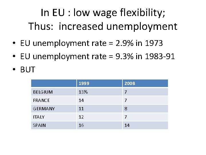
In EU : low wage flexibility; Thus: increased unemployment • EU unemployment rate = 2. 9% in 1973 • EU unemployment rate = 9. 3% in 1983 -91 • BUT 1999 2008 BELGIUM 13% 7 FRANCE 14 7 GERMANY 11 8 ITALY 12 7 SPAIN 16 14

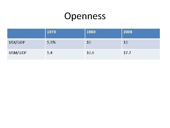
Openness 1970 1980 2008 USX/GDP 5. 5% 10 13 USM/GDP 5. 4 10. 6 17. 7

Trade and Income Inequality • 1. most studies find a link but not a major factor for increased inequality. • 2. Counter-evidence: Stolper-Samuelson predicts: price of unskilled-labor-intensive products to decline relative to price of skilledlab-int or K-int products. • This is NOT OBSERVED.

• 3. In developed countries: demand for skilled labor increased relative to demand for unskilled labor. • This IS TRUE even for NON-TRADED Sectors. • 4. Technology may increase Income Inequality: • Fed Reserve of NY estimate: • Technology contribute to 45% increase in Inequal. • Trade contribute to 11% of increase in Inequality

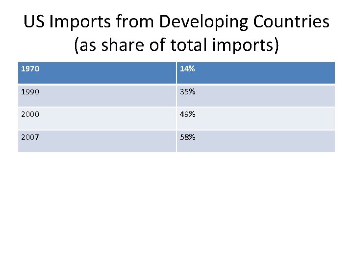
US Imports from Developing Countries (as share of total imports) 1970 14% 1990 35% 2000 49% 2007 58%