Lens Design Lectures 4 5 OPTI 517 College

Lens Design Lectures 4 -5 OPTI 517 College of Optical Sciences University of Arizona

Tolerance Analysis

In the computer • So far, the designs have been “on paper” (OK: in computer) – Predesign based on “paraxial” properties – Optimization to minimize optical aberrations • Assume rotational symmetry – Final design exceeds minimum performance requirements • Performance of real systems will not match computer simulation – Manufacturing errors and limitations – Real systems ALWAYS are degraded relative to ideal design • These degradations may significantly reduce the overall quality of the design Copyright 2017 Mary G. Turner 3

What is a tolerance analysis • A statistical process that systematically introduces specific aberrations or perturbations into an optical design to determine the impact on system performance • Perturbations are applied to all optical and mechanical dimensions and parameters to determine the overall tolerance budget • Determine the amounts of various types of errors that are allowed in manufacture and assembly so that the final system has some defined statistical likelihood of performing to the level of the design goal Copyright 2017 Mary G. Turner 4

Why perform tolerance analysis? • Tolerancing assumes reality: – No optic is perfectly polished – No mechanical mount is perfectly machined – Each glass melt has some variations – No system is perfectly assembled • The real question: – How close to the design specifications does the system need to be? Keep in mind: A design can only perform to the level it is actually manufactured Copyright 2017 Mary G. Turner 5

Who performs the analysis? • Each optical designer is responsible for the proper tolerancing of their individual designs – No one else fully understands the thought process of the design • It is not the responsibility of the optical fabricator or the mechanical design team to make the system work • The fundamental design must have sufficient freedom to work within reasonable manufacturing limits • The best design may not be the system with the lowest merit function value: – It is the design that can be built to best meet the design requirements Copyright 2017 Mary G. Turner 6

Goal of tolerance analysis • Determine appropriate tolerance ranges for all optical and mechanical components: – Lenses, mirrors, windows, filters – Mechanical mounts, spacers, apertures • Optical performance criteria met with: – Minimum cost for optics – Minimum cost and complexity in assembly and alignment – Maximum yield • Process differs slightly for mass produced systems and oneoffs, but tolerance analysis must always be performed Copyright 2017 Mary G. Turner 7

Test plate fitting • Last step of design or first step of tolerancing: – Most optical fabricators have an inventory of test plates: • CC and CX surfaces polished and measured to high accuracy • Used to compare surfaces being made • Reoptimizing design to match available test plates saves time and money – Zemax includes test plate lists for many manufacturers • Match radius with Diameter at least to CA size • You can also make your own • Note: Test plates are made of glass – Always verify with the fabricators that the test plates needed are still available Copyright 2017 Mary G. Turner 8

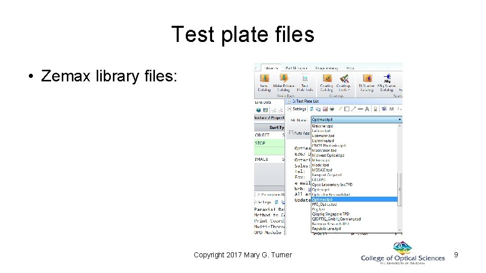
Test plate files • Zemax library files: Copyright 2017 Mary G. Turner 9

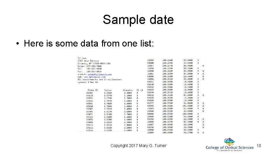
Sample date • Here is some data from one list: Copyright 2017 Mary G. Turner 10

Plate fit process • Start with a lens in final design form • Leave all radii to be fit variable – Remove any radius solves and replace with MF constraint • Leave as many "compensators" free as possible – Let thickness’ vary (within bounds: should not change much) • Different options to fitting the test plates • Best first, worst first, Long first, short first, Try all – Finds radii with best match to a test plate radii (If best first method) • Uses "fringes" as criterion for fit – Sets that radii to the exact TP radii, removes variability – Reoptimize – Repeat until all radii are matched (if possible) Copyright 2017 Mary G. Turner 11

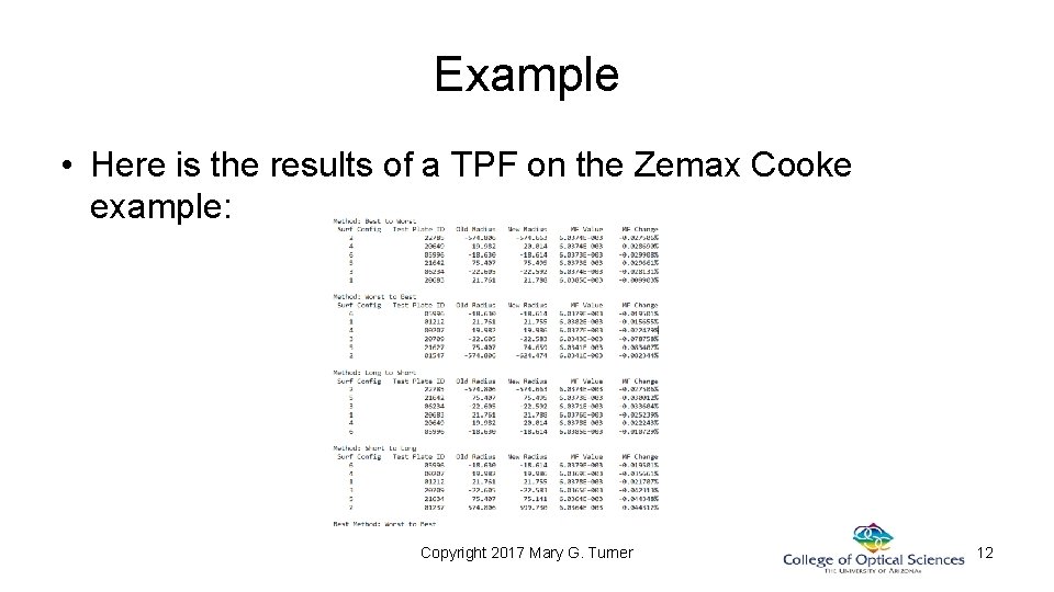
Example • Here is the results of a TPF on the Zemax Cooke example: Copyright 2017 Mary G. Turner 12

File updated • The information in the LDE matches the best fit – Undo to go back – Save file (new name) to keep – Contact optical fab shop to verify plates • Sometimes TPF fails for one or more surface: – Introduced error too large – Perform a fit “by hand” for problem surfaces – May need custom plate or interferometric testing • Add cost, and time Copyright 2017 Mary G. Turner 13

TPF considerations • TPF is done to the plates of a specific fabricator – May not have the best plates for a specific design • Sometimes restricted to specific vendor – Do not sacrifice system performance for test plate fitting • That further reduces available error for tolerancing • TPF benefit: – When measured compared to a test plate, the error in the surface curvature can be known to a tighter tolerance than it could otherwise be measured Copyright 2017 Mary G. Turner 14

Last pre-step • Now do something similar for lens thicknesses: – Adjust thickness values for nnnn. nn (two decimal places) – One at a time – Reoptimize – Adjust next – Continue until completed – If problem surface, make other thickness values variable the readjust Copyright 2017 Mary G. Turner 15

Tolerancing procedure • Assign reasonable initial tolerance ranges to all optical and mechanical components – Reasonable: easily attained in fabrication: “Commercial” – Zemax has defaults (make necessary adjustments) • Determine the appropriate "figure of merit" for use as a tolerance criteria – Usually related to design MF • RMS spot size, RMS wavefront error, MTF requirement, User defined merit function, boresight, etc. • Determine how much the system performance can depart from “paper” performance Copyright 2017 Mary G. Turner 16

And then • Identify compensators to be used to relax the tolerances – At least one compensator, usually the back focus, is used • Evaluate the each tolerance to estimate the expected change in performance – Three types of analysis are available: • Sensitivity • Inverse Sensitivity • Monte Carlo • Revise tolerance ranges to meet error "budget" • Repeat until required performance level is reached at reasonable cost Copyright 2017 Mary G. Turner 17

Error Sources and Budget

Sources of error • Several types of errors need to be considered: – Errors in fabrication – Errors in material properties (index, Abbe) – Errors in the assembly of the system – Errors due to thermal (and other environmental) conditions – Errors in “paper” design Copyright 2017 Mary G. Turner 19

Errors in fabrication • These include: – Errors in radius of curvature – Errors in center thickness – Error in surface shape – Offset of center of curvature from mechanical center – Errors in conics or higher order aspherics (or other surface parameters) Copyright 2017 Mary G. Turner 20

Errors in materials • Batch to batch variations in glass properties: – Index variation from nominal – Index homogeneity – Homogeneity gradient – Dispersion variations • Measurements can be made to very high accuracy Copyright 2017 Mary G. Turner 21

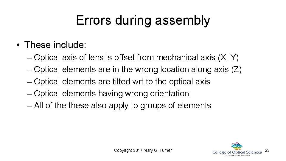
Errors during assembly • These include: – Optical axis of lens is offset from mechanical axis (X, Y) – Optical elements are in the wrong location along axis (Z) – Optical elements are tilted wrt to the optical axis – Optical elements having wrong orientation – All of these also apply to groups of elements Copyright 2017 Mary G. Turner 22

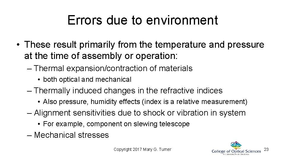
Errors due to environment • These result primarily from the temperature and pressure at the time of assembly or operation: – Thermal expansion/contraction of materials • both optical and mechanical – Thermally induced changes in the refractive indices • Also pressure, humidity effects (index is a relative measurement) – Alignment sensitivities due to shock or vibration in system • For example, component on slewing telescope – Mechanical stresses Copyright 2017 Mary G. Turner 23

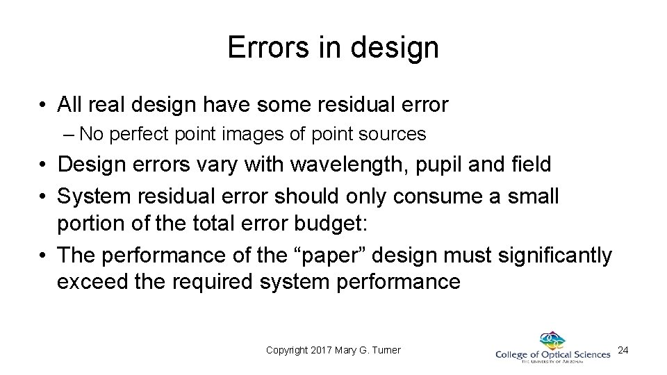
Errors in design • All real design have some residual error – No perfect point images of point sources • Design errors vary with wavelength, pupil and field • System residual error should only consume a small portion of the total error budget: • The performance of the “paper” design must significantly exceed the required system performance Copyright 2017 Mary G. Turner 24

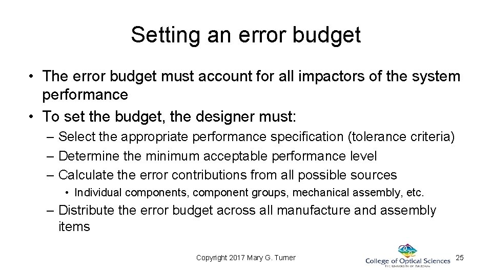
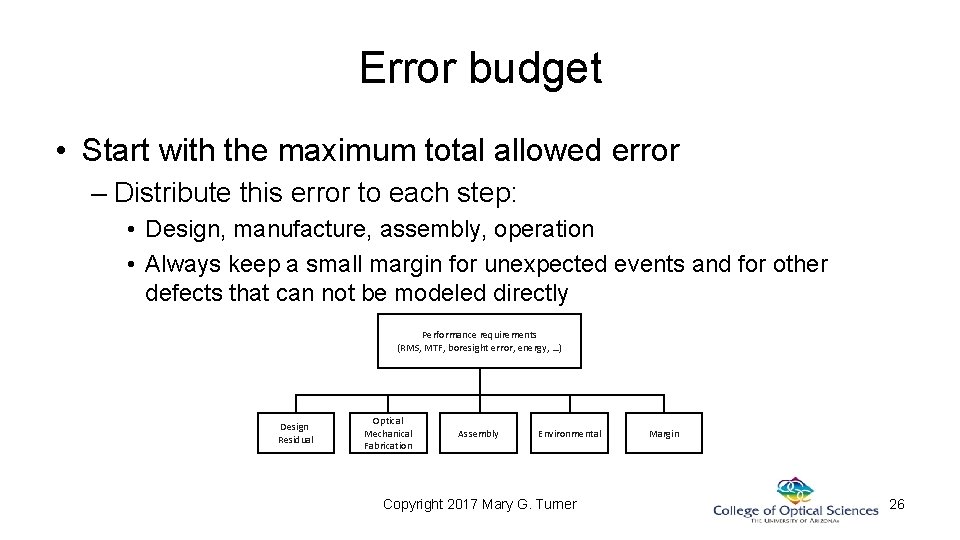
Setting an error budget • The error budget must account for all impactors of the system performance • To set the budget, the designer must: – Select the appropriate performance specification (tolerance criteria) – Determine the minimum acceptable performance level – Calculate the error contributions from all possible sources • Individual components, component groups, mechanical assembly, etc. – Distribute the error budget across all manufacture and assembly items Copyright 2017 Mary G. Turner 25

Error budget • Start with the maximum total allowed error – Distribute this error to each step: • Design, manufacture, assembly, operation • Always keep a small margin for unexpected events and for other defects that can not be modeled directly Performance requirements (RMS, MTF, boresight error, energy, …) Design Residual Optical Mechanical Fabrication Assembly Environmental Copyright 2017 Mary G. Turner Margin 26

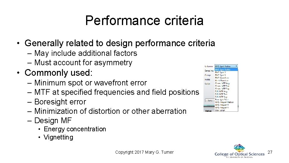
Performance criteria • Generally related to design performance criteria – May include additional factors – Must account for asymmetry • Commonly used: – Minimum spot or wavefront error – MTF at specified frequencies and field positions – Boresight error – Minimization of distortion or other aberration – Design MF • Energy concentration • Vignetting Copyright 2017 Mary G. Turner 27

Sensitivity analysis • Copyright 2017 Mary G. Turner 28

Inverse sensitivity analysis • The sensitivity analysis will generally indicate that some of the tolerance ranges are too loose to allow for acceptable system performance • Inverse sensitivity analysis is used selectively tighter ranges: – Establish maximum criteria change, what is the parameter range? – A series of individual tolerance operands are evaluated • For each operand, any compensators are adjusted to minimize the performance criterion. Each tolerance limit is iteratively adjusted until the change in performance is equal to a preset maximum degradation. – Tolerances which meet the criteria are not loosened. – Report listing the results is displayed Copyright 2017 Mary G. Turner 29

Monte Carlo analysis • Sensitivity and inverse sensitivity analyze each parameter at the limits of its tolerance range • Statistical summing of data gives “worst case” scenario • Monte Carlo simulation considers all parameters – Each parameter is perturbed within its tolerance limits – Statistical distribution of errors • Random systems are generated • Any compensators are used to optimize • Again, a massive report is produced Copyright 2017 Mary G. Turner 30

Error statistics • Statistical distributions available for use during MC analysis: – Gaussian(Normal): • Selects offset assuming the 1/e point on the bell curve is ¼ the distance between the min and max values. Width may be altered by the user. – Uniform: • Selects offset with equal probability anywhere between the min and max – Parabolic: • Selects offset with quadratic probability, favors the ends of the range – User Defined: • Select values using any arbitrary user-defined probability distribution • Different statistics may be applied to different parameters or in different situations Copyright 2017 Mary G. Turner 31

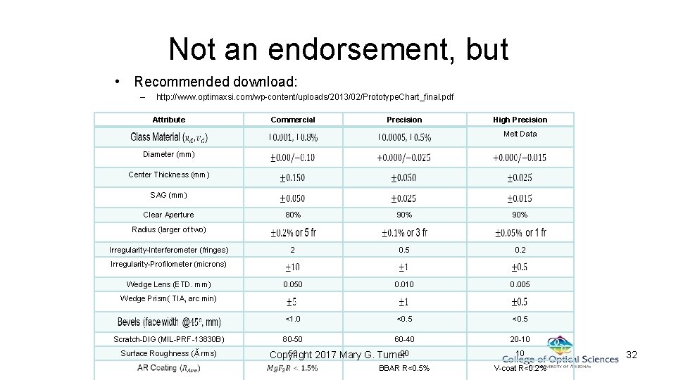
Not an endorsement, but • Recommended download: – http: //www. optimaxsi. com/wp-content/uploads/2013/02/Prototype. Chart_final. pdf Attribute Commercial Precision High Precision Melt Data Diameter (mm) Center Thickness (mm) SAG (mm) Clear Aperture 80% 90% 2 0. 5 0. 2 0. 050 0. 010 0. 005 <1. 0 <0. 5 80 -50 60 -40 20 -10 Radius (larger of two) Irregularity-Interferometer (fringes) Irregularity-Profilometer (microns) Wedge Lens (ETD. mm) Wedge Prism( TIA, arc min) Scratch-DIG (MIL-PRF-13830 B) Surface Roughness (Ặ rms) 50 20 Copyright 2017 Mary G. Turner BBAR R<0. 5% 10 V-coat R<0. 2% 32

Tolerance range • Start with reasonable tolerances, the previous page lists some good starting points, but: – Talk to your optical fabricator – Talk to your mechanical design team • Properly performed tolerancing will allow an estimation of the system performance: – If 1000 of these systems are built, 95% will have an on-axis MTF greater than 50% at 30 lpm, and greater than 30% at 50 lpm – Cost comparisons can be done to other success rates such as 90% and 98% – For one-off systems, the percentage amounts to the likelihood the single system will work Copyright 2017 Mary G. Turner 33

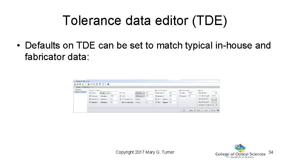
Tolerance data editor (TDE) • Defaults on TDE can be set to match typical in-house and fabricator data: Copyright 2017 Mary G. Turner 34

Copyright 2017 Mary G. Turner 35

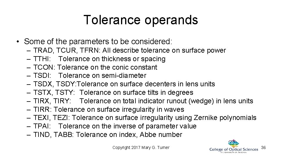
Tolerance operands • Some of the parameters to be considered: – – – TRAD, TCUR, TFRN: All describe tolerance on surface power TTHI: Tolerance on thickness or spacing TCON: Tolerance on the conic constant TSDI: Tolerance on semi-diameter TSDX, TSDY: Tolerance on surface decenters in lens units TSTX, TSTY: Tolerance on surface tilts in degrees TIRX, TIRY: Tolerance on total indicator runout (wedge) in lens units TIRR: Tolerance on surface irregularity in waves TEXI, TEZI: Tolerance on surface irregularity using Zernike polynomials TPAI: Tolerance on the inverse of parameter value TIND, TABB: Tolerance on index, Abbe number Copyright 2017 Mary G. Turner 36

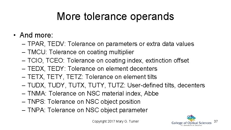
More tolerance operands • And more: – TPAR, TEDV: Tolerance on parameters or extra data values – TMCU: Tolerance on coating multiplier – TCIO, TCEO: Tolerance on coating index, extinction offset – TEDX, TEDY: Tolerance on element decenters – TETX, TETY, TETZ: Tolerance on element tilts – TUDX, TUDY, TUTX, TUTY, TUTZ: User-defined tilts, decenters – TNMA: Tolerance on NSC material index, Abbe – TNPS: Tolerance on NSC object position – TNPA: Tolerance on NSC object parameter Copyright 2017 Mary G. Turner 37

One lens at a time • Sources of error in a singlet lens: – Each surface has the wrong power – Center thickness is wrong – Optical and mechanical axes of the surfaces are offset – Surfaces can be wedged – Surfaces are not spherical – Index of the material is different from nominal – Index varies within the lens – Abbe dispersion value is incorrect • Use a singlet to understand the operands Copyright 2017 Mary G. Turner 38

TRAD, TCUR, TFRN • Any of these operands can be used to set the tolerance range on surface power • If tests plates are used, error will be measured wrt test plate, in fringes • Power change is proportion to Δc, but not to ΔR • We tend to think in radius, not curvature • All of these represent the same error. Apply one to a given surface Copyright 2017 Mary G. Turner 39

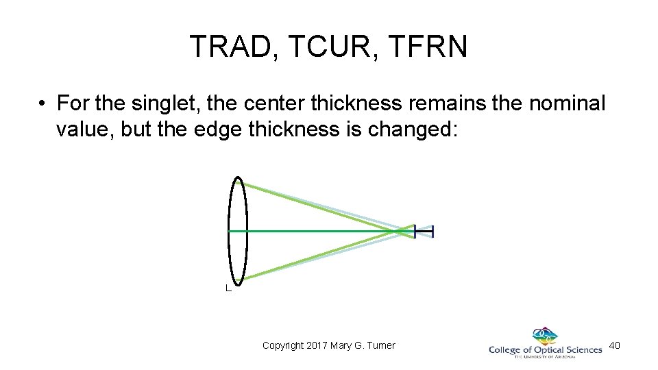
TRAD, TCUR, TFRN • For the singlet, the center thickness remains the nominal value, but the edge thickness is changed: Copyright 2017 Mary G. Turner 40

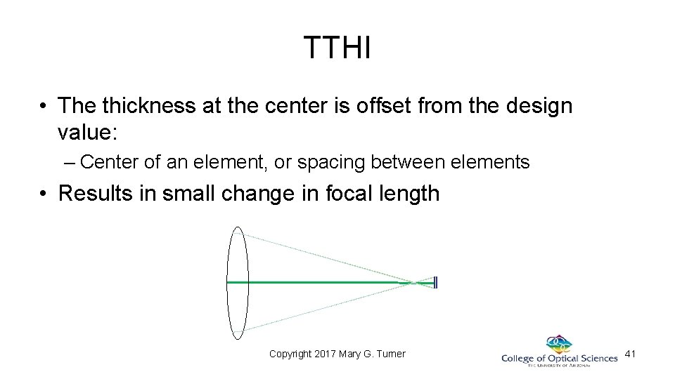
TTHI • The thickness at the center is offset from the design value: – Center of an element, or spacing between elements • Results in small change in focal length Copyright 2017 Mary G. Turner 41

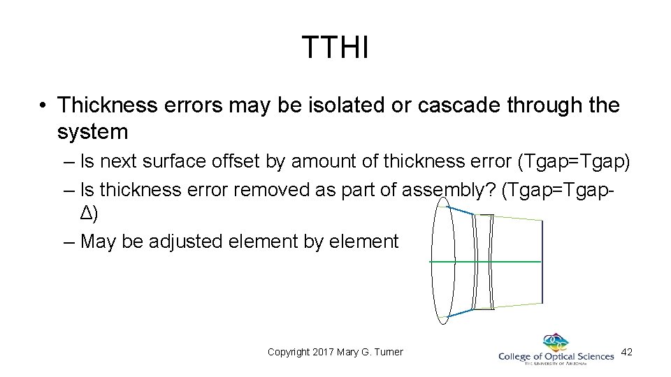
TTHI • Thickness errors may be isolated or cascade through the system – Is next surface offset by amount of thickness error (Tgap=Tgap) – Is thickness error removed as part of assembly? (Tgap=TgapΔ) – May be adjusted element by element Copyright 2017 Mary G. Turner 42

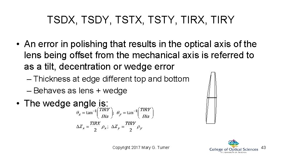
TSDX, TSDY, TSTX, TSTY, TIRX, TIRY • An error in polishing that results in the optical axis of the lens being offset from the mechanical axis is referred to as a tilt, decentration or wedge error – Thickness at edge different top and bottom – Behaves as lens + wedge • The wedge angle is: Copyright 2017 Mary G. Turner 43

TSDX, TSDY, TSTX, TSTY, TIRX, TIRY • Tolerance this effect once per component • Typically applied to one side of the element only: – Optics polished so one surface defines the center and the second surface is wedged relative to that surface • For spherical surfaces, the effect of a surface decenter is the same as a surface tilt • For conics and aspheres, these represent separate tolerances Copyright 2017 Mary G. Turner 44

TIRR, TEXI, TEZI • Surface irregularity refers to a non-spherical shape for a nominally spherical surface – The surface contributes additional aberration to the optical design • Two methods of modeling surface irregularity are available: – Irregularity composed of spherical aberration and astigmatism • Low order aberration terms – Irregularity represented as a sum of Zernike terms • Higher order aberrations Copyright 2017 Mary G. Turner 45

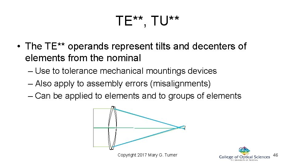
TE**, TU** • The TE** operands represent tilts and decenters of elements from the nominal – Use to tolerance mechanical mountings devices – Also apply to assembly errors (misalignments) – Can be applied to elements and to groups of elements Copyright 2017 Mary G. Turner 46

Compensators • Key parameter in tolerancing – A specified design parameter used to offset the effect of errors in other parameters – The ability to compensate for the errors introduced in manufacturing and assembly allows for wider tolerance ranges • Higher likelihood of success • Much lower cost – Most common compensator is image plane location: • Several errors (TFRN, TTHI, TIND and others) resulted primarily in a change in power: – Compensate by finding the new “best focus” Copyright 2017 Mary G. Turner 47

When do you use compensators? • Since compensators allow larger tolerances ranges, they can reduce costs – Always good • In addition to back focal distance, commonly used include: – Tilt of focal plane to compensate for asymmetric errors • Think back to discussion of coma – Decentration of the focal plane (chief ray alignment: boresight) • Compensators are degrees of freedom, usually applied mechanically: – Check with mechanical department in advance Copyright 2017 Mary G. Turner 48

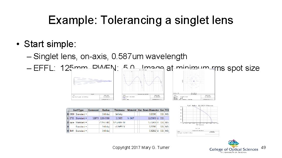
Example: Tolerancing a singlet lens • Start simple: – Singlet lens, on-axis, 0. 587 um wavelength – EFFL: 125 mm PWFN: 5. 0, Image at minimum rms spot size Copyright 2017 Mary G. Turner 49

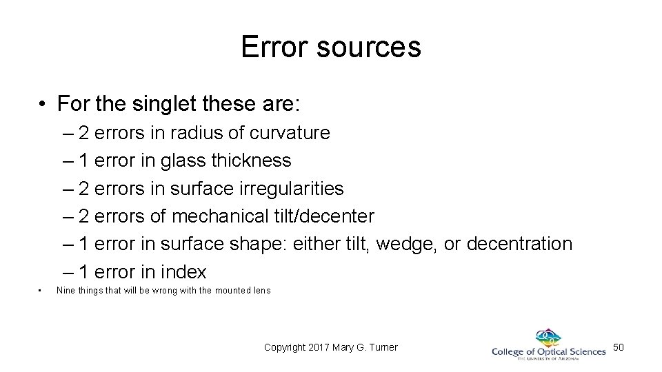
Error sources • For the singlet these are: – 2 errors in radius of curvature – 1 error in glass thickness – 2 errors in surface irregularities – 2 errors of mechanical tilt/decenter – 1 error in surface shape: either tilt, wedge, or decentration – 1 error in index • Nine things that will be wrong with the mounted lens Copyright 2017 Mary G. Turner 50

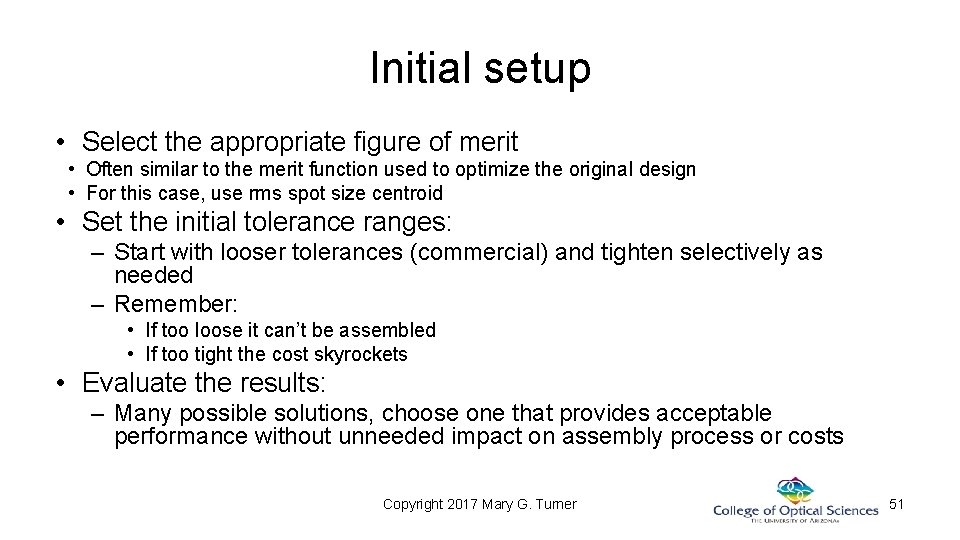
Initial setup • Select the appropriate figure of merit • Often similar to the merit function used to optimize the original design • For this case, use rms spot size centroid • Set the initial tolerance ranges: – Start with looser tolerances (commercial) and tighten selectively as needed – Remember: • If too loose it can’t be assembled • If too tight the cost skyrockets • Evaluate the results: – Many possible solutions, choose one that provides acceptable performance without unneeded impact on assembly process or costs Copyright 2017 Mary G. Turner 51

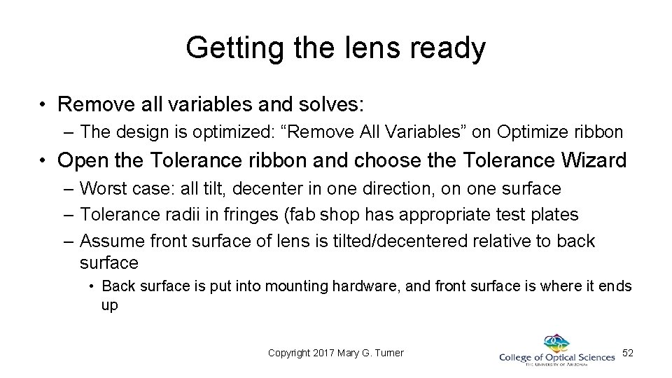
Getting the lens ready • Remove all variables and solves: – The design is optimized: “Remove All Variables” on Optimize ribbon • Open the Tolerance ribbon and choose the Tolerance Wizard – Worst case: all tilt, decenter in one direction, on one surface – Tolerance radii in fringes (fab shop has appropriate test plates – Assume front surface of lens is tilted/decentered relative to back surface • Back surface is put into mounting hardware, and front surface is where it ends up Copyright 2017 Mary G. Turner 52

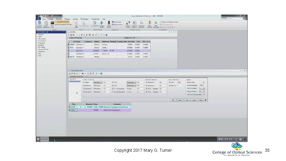
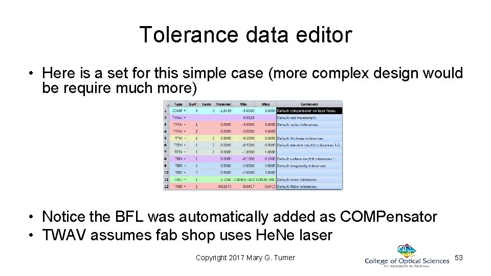
Tolerance data editor • Here is a set for this simple case (more complex design would be require much more) • Notice the BFL was automatically added as COMPensator • TWAV assumes fab shop uses He. Ne laser Copyright 2017 Mary G. Turner 53

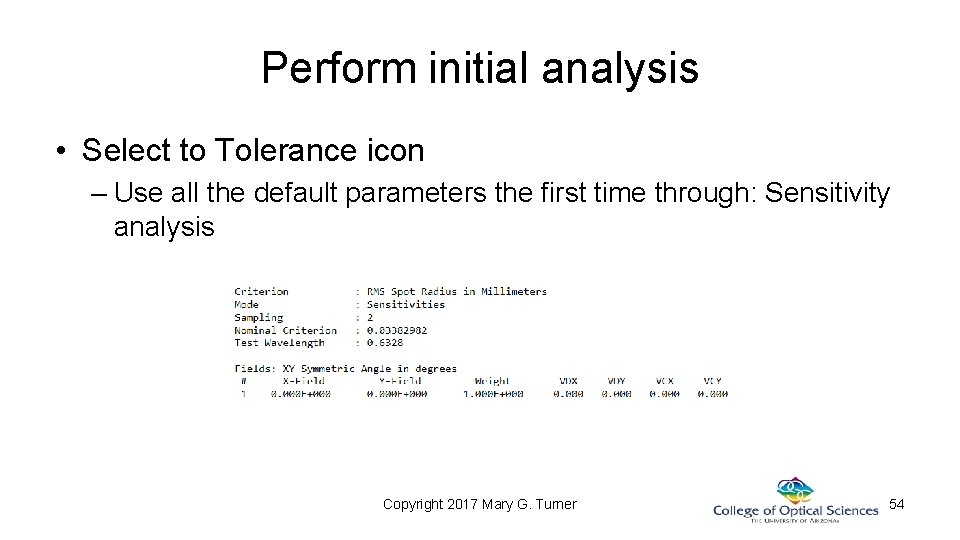
Perform initial analysis • Select to Tolerance icon – Use all the default parameters the first time through: Sensitivity analysis Copyright 2017 Mary G. Turner 54

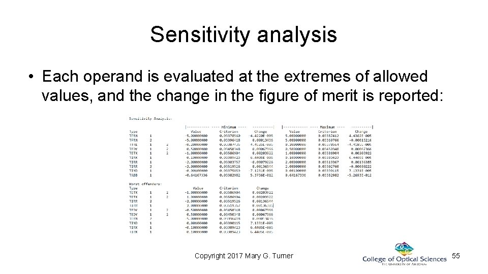
Sensitivity analysis • Each operand is evaluated at the extremes of allowed values, and the change in the figure of merit is reported: Copyright 2017 Mary G. Turner 55

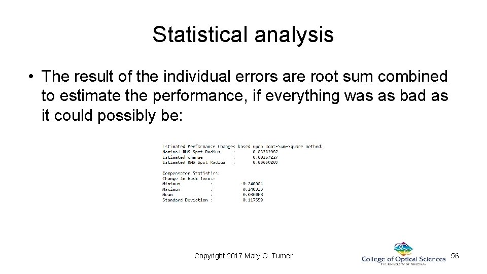
Statistical analysis • The result of the individual errors are root sum combined to estimate the performance, if everything was as bad as it could possibly be: Copyright 2017 Mary G. Turner 56

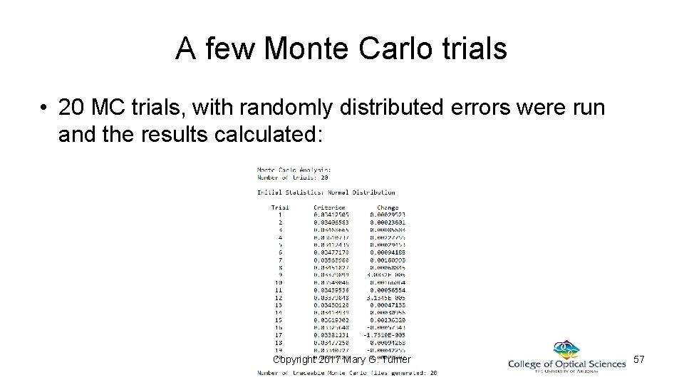
A few Monte Carlo trials • 20 MC trials, with randomly distributed errors were run and the results calculated: Copyright 2017 Mary G. Turner 57

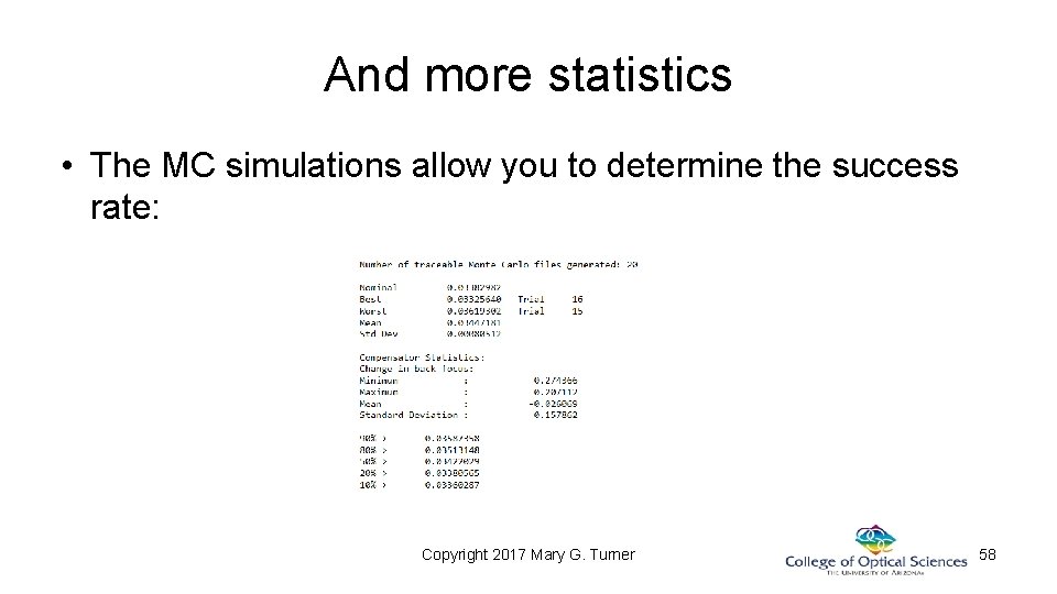
And more statistics • The MC simulations allow you to determine the success rate: Copyright 2017 Mary G. Turner 58

For small quantities • For one-off systems, or for a small number of systems, use worst case simulations: – Statistics can never give 100% likelihood, but • A 95% success rate if everything goes wrong is much more comforting than a 98% success rate if everything goes perfectly Copyright 2017 Mary G. Turner 59

In mass production • This is where MC analysis provides most information • Use MC analysis generates as many different designs as needed to estimate the percentage of systems that will meet (or exceed) the performance specification. – Number of runs should be (number of operands)^2 • Can usually get by with smaller number • ZEMAX reports the value of each compensator, as well as the minimum and maximum values. – This is needed by manufacturing. A compensator is a mechanical or other adjustment. Copyright 2017 Mary G. Turner 60