Lemkes Algorithm The Hammer in Your Math Toolbox

Lemke’s Algorithm: The Hammer in Your Math Toolbox? Chris Hecker definition six, inc. checker@d 6. com 1

First, a Word About Hammers “If the only tool you have is a hammer, you tend to see every problem as a nail. ” Abraham Maslow • requirements for this to be a good idea • a way of transforming problems into nails (MLCPs) • a hammer (Lemke’s algorithm) • lots of advanced info + one hour = something has to give • majority of lecture is motivating you to care about the hammer by showing you how useful nails can be • make you hunger for more info post-lecture • very little on how the hammer works in this hour 2

Hammers (cont. ) • by definition, not the optimal way to solve problems, BUT – computers are very fast these days – often don’t care about optimality • prepro, prototypes, tools, not a profile hotspot, etc. – can always move to optimal solution after you verify it’s a problem you actually want to solve 3

What are “advanced game math problems”? • problems that are ammenable to mathematical modeling • state the problem clearly • state the desired solution clearly • describe the problem with equations so a proposed solution’s quality is measurable • figure out how to solve the equations • why not hack it? • I believe better modeling is the future of game technology development (consistency, not reality) 4

Prerequisites • linear algebra • vector, matrix symbol manipulation at least • calculus concepts • what derivatives mean • comfortable with math notation and concepts 5

Overview of Lecture • random assortment of example problems breifly mentioned • 5 specific example problems in some depth • including one that I ran into recently and how I solved it • generalize the example models • transform them all to MLCPs • solve MLCPs with Lemke’s algorithm 6

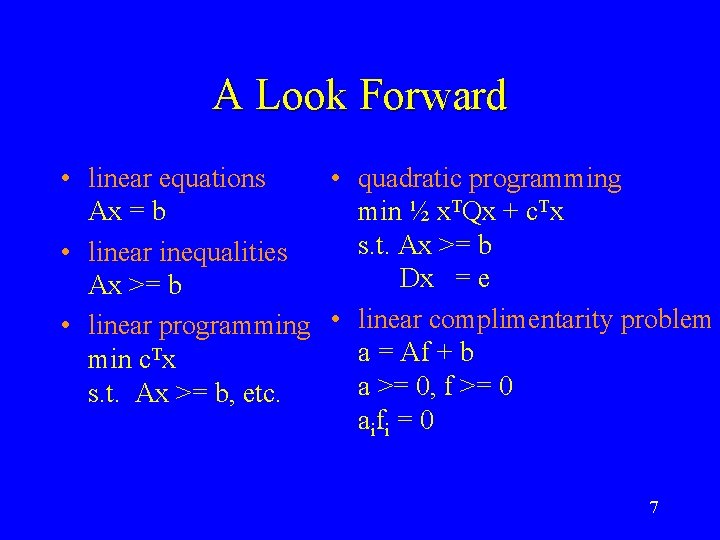
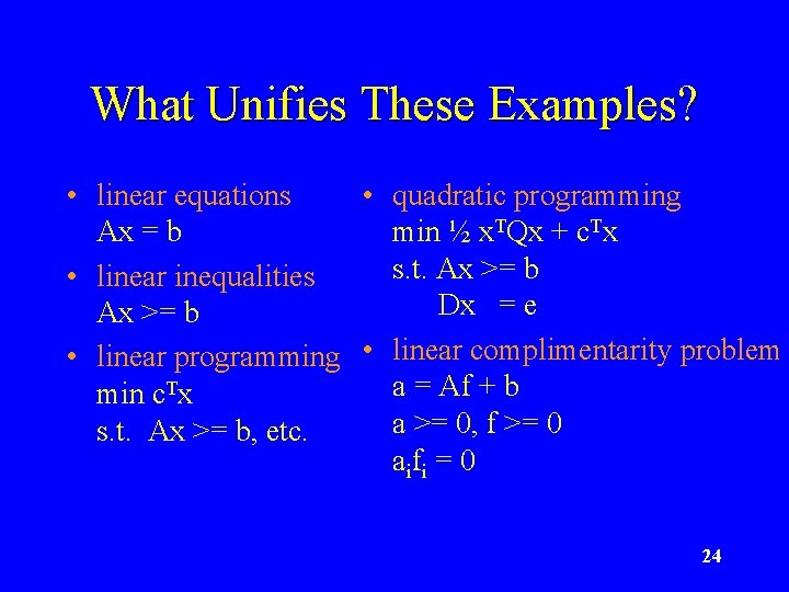
A Look Forward • linear equations • quadratic programming Ax = b min ½ x. TQx + c. Tx s. t. Ax >= b • linear inequalities Dx = e Ax >= b • linear programming • linear complimentarity problem a = Af + b min c. Tx a >= 0, f >= 0 s. t. Ax >= b, etc. a i fi = 0 7

Applications to Games graphics, physics, ai, even ui • • computational geometry visibility contact curve fitting constraints integration graph theory • • network flow economics site allocation game theory IK machine learning image processing 8

Applications to Games (cont. ) • don’t forget. . . – The Elastohydrodynamic Lubrication Problem – Solving Optimal Ownership Structures • “The two parties establish a relationship in which they exchange feed ingredients, q, and manure, m. ” 9

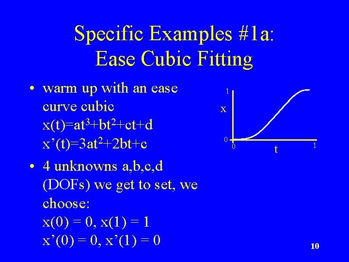
Specific Examples #1 a: Ease Cubic Fitting • warm up with an ease curve cubic x(t)=at 3+bt 2+ct+d x’(t)=3 at 2+2 bt+c • 4 unknowns a, b, c, d (DOFs) we get to set, we choose: x(0) = 0, x(1) = 1 x’(0) = 0, x’(1) = 0 1 x 0 0 t 1 10

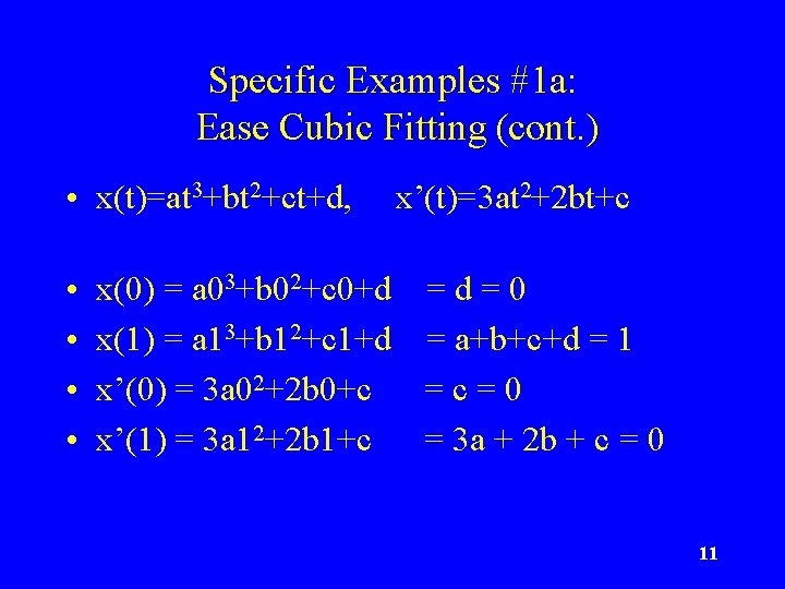
Specific Examples #1 a: Ease Cubic Fitting (cont. ) • x(t)=at 3+bt 2+ct+d, • • x’(t)=3 at 2+2 bt+c x(0) = a 03+b 02+c 0+d = 0 x(1) = a 13+b 12+c 1+d = a+b+c+d = 1 x’(0) = 3 a 02+2 b 0+c =c=0 x’(1) = 3 a 12+2 b 1+c = 3 a + 2 b + c = 0 11

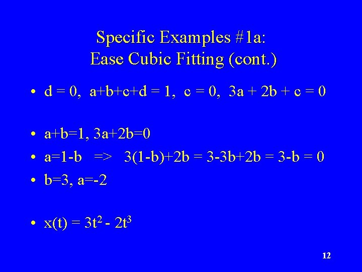
Specific Examples #1 a: Ease Cubic Fitting (cont. ) • d = 0, a+b+c+d = 1, c = 0, 3 a + 2 b + c = 0 • a+b=1, 3 a+2 b=0 • a=1 -b => 3(1 -b)+2 b = 3 -3 b+2 b = 3 -b = 0 • b=3, a=-2 • x(t) = 3 t 2 - 2 t 3 12

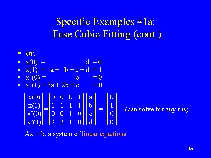
Specific Examples #1 a: Ease Cubic Fitting (cont. ) • or, • • x(0) = d x(1) = a + b + c + d x’(0) = c x’(1) = 3 a + 2 b + c x(0) 0 0 x(1) 1 1 = x’(0) 0 0 x’(1) 3 2 0 1 1 1 0 0 =0 =1 =0 =0 a b = c d 0 1 0 0 (can solve for any rhs) Ax = b, a system of linear equations 13

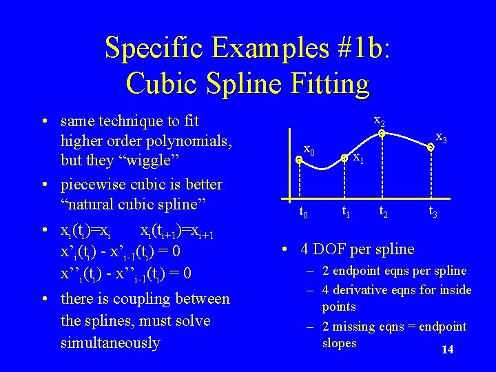
Specific Examples #1 b: Cubic Spline Fitting • same technique to fit higher order polynomials, but they “wiggle” • piecewise cubic is better “natural cubic spline” • xi(ti)=xi xi(ti+1)=xi+1 x’i(ti) - x’i-1(ti) = 0 x’’i(ti) - x’’i-1(ti) = 0 • there is coupling between the splines, must solve simultaneously x 2 x 0 t 0 x 3 x 1 t 2 t 3 • 4 DOF per spline – 2 endpoint eqns per spline – 4 derivative eqns for inside points – 2 missing eqns = endpoint slopes 14

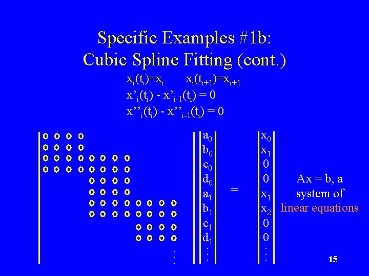
Specific Examples #1 b: Cubic Spline Fitting (cont. ) xi(ti)=xi xi(ti+1)=xi+1 x’i(ti) - x’i-1(ti) = 0 x’’i(ti) - x’’i-1(ti) = 0 . . . a 0 b 0 c 0 d 0 a 1 b 1 c 1 d 1. . . = x 0 x 1 0 Ax = b, a 0 system of x 1 x 2 linear equations 0 0. . . 15

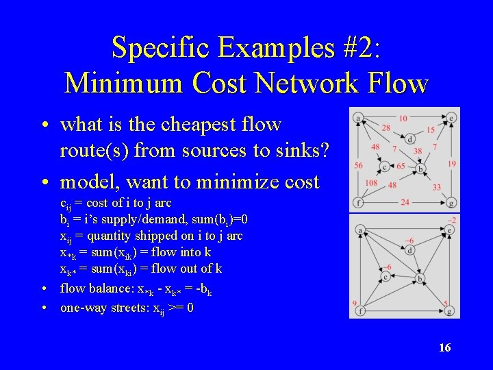
Specific Examples #2: Minimum Cost Network Flow • what is the cheapest flow route(s) from sources to sinks? • model, want to minimize cost cij = cost of i to j arc bi = i’s supply/demand, sum(bi)=0 xij = quantity shipped on i to j arc x*k = sum(xik) = flow into k xk* = sum(xki) = flow out of k • flow balance: x*k - xk* = -bk • one-way streets: xij >= 0 16

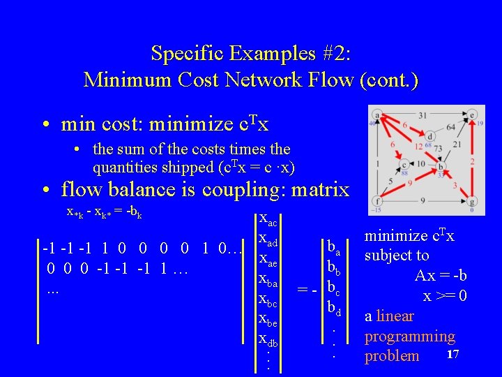
Specific Examples #2: Minimum Cost Network Flow (cont. ) • min cost: minimize c. Tx • the sum of the costs times the quantities shipped (c. Tx = c ·x) • flow balance is coupling: matrix x*k - xk* = -bk xac xad -1 -1 -1 1 0 0 1 0… xae 0 0 0 -1 -1 -1 1 … xba. . . xbc xbe xdb. . . ba bb = - bc bd. . . minimize c. Tx subject to Ax = -b x >= 0 a linear programming 17 problem

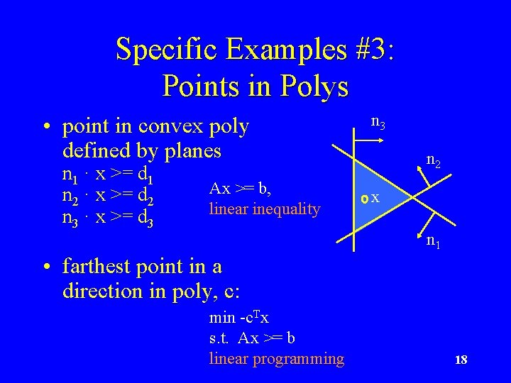
Specific Examples #3: Points in Polys • point in convex poly defined by planes n 1 · x >= d 1 n 2 · x >= d 2 n 3 · x >= d 3 Ax >= b, linear inequality n 3 n 2 x n 1 • farthest point in a direction in poly, c: min -c. Tx s. t. Ax >= b linear programming 18

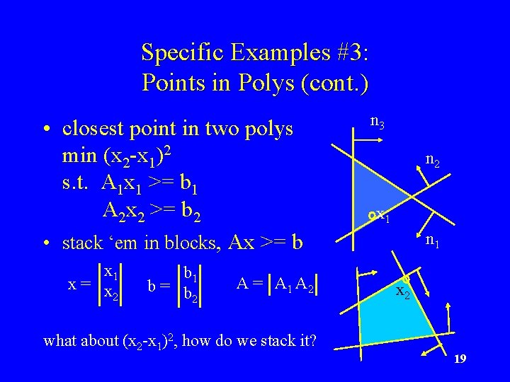
Specific Examples #3: Points in Polys (cont. ) • closest point in two polys min (x 2 -x 1)2 s. t. A 1 x 1 >= b 1 A 2 x 2 >= b 2 • stack ‘em in blocks, Ax >= b x 1 x= x 2 b 1 b= b 2 A = A 1 A 2 what about (x 2 -x 1)2, how do we stack it? n 3 n 2 x 1 n 1 x 2 19

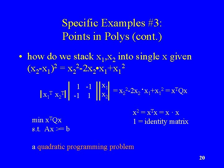
Specific Examples #3: Points in Polys (cont. ) • how do we stack x 1, x 2 into single x given (x 2 -x 1)2 = x 22 -2 x 2 • x 1+x 12 x 1 T x 2 T min x. TQx s. t. Ax >= b 1 -1 -1 1 x 1 2 -2 x • x +x 2 = x. TQx = x 2 2 1 1 x 2 = x. Tx = x · x 1 = identity matrix a quadratic programming problem 20

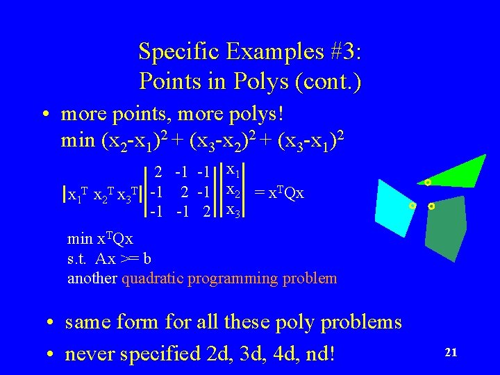
Specific Examples #3: Points in Polys (cont. ) • more points, more polys! min (x 2 -x 1)2 + (x 3 -x 2)2 + (x 3 -x 1)2 x 1 T x 2 T x 3 T 2 -1 -1 x 1 -1 2 -1 x 2 = x. TQx -1 -1 2 x 3 min x. TQx s. t. Ax >= b another quadratic programming problem • same form for all these poly problems • never specified 2 d, 3 d, 4 d, nd! 21

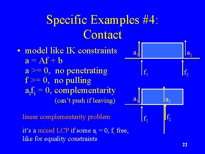
Specific Examples #4: Contact • model like IK constraints a = Af + b a >= 0, no penetrating f >= 0, no pulling aifi = 0, complementarity (can’t push if leaving) linear complementarity problem it’s a mixed LCP if some ai = 0, fi free, like for equality constraints a 1 a 2 f 1 a 1 f 2 a 2 f 1 f 2 22

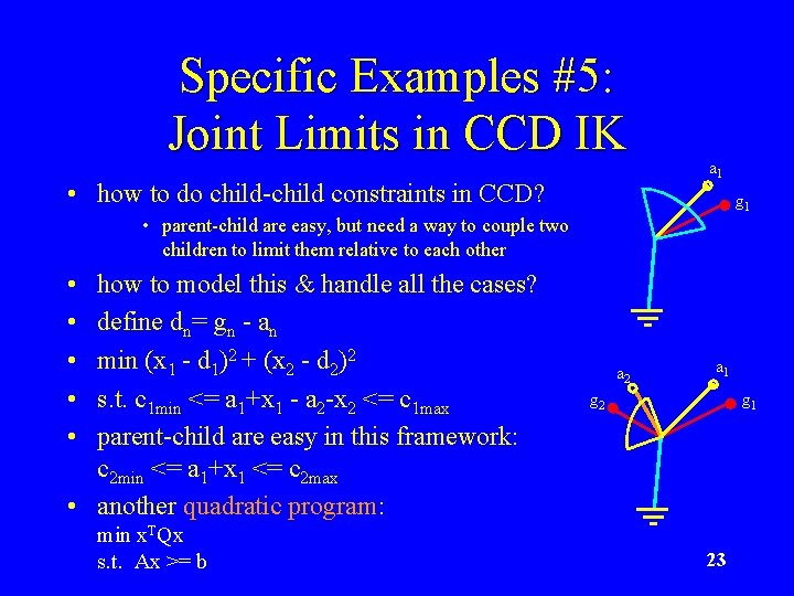
Specific Examples #5: Joint Limits in CCD IK • how to do child-child constraints in CCD? a 1 g 1 • parent-child are easy, but need a way to couple two children to limit them relative to each other • • • how to model this & handle all the cases? define dn= gn - an min (x 1 - d 1)2 + (x 2 - d 2)2 s. t. c 1 min <= a 1+x 1 - a 2 -x 2 <= c 1 max parent-child are easy in this framework: c 2 min <= a 1+x 1 <= c 2 max • another quadratic program: min x. TQx s. t. Ax >= b a 2 a 1 g 2 g 1 23

What Unifies These Examples? • linear equations • quadratic programming Ax = b min ½ x. TQx + c. Tx s. t. Ax >= b • linear inequalities Dx = e Ax >= b • linear programming • linear complimentarity problem a = Af + b min c. Tx a >= 0, f >= 0 s. t. Ax >= b, etc. a i fi = 0 24

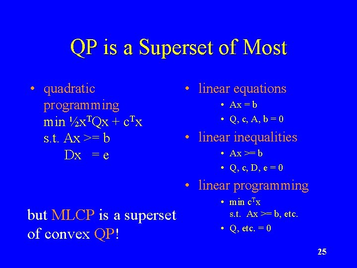
QP is a Superset of Most • quadratic programming min ½x. TQx + c. Tx s. t. Ax >= b Dx = e • linear equations • Ax = b • Q, c, A, b = 0 • linear inequalities • Ax >= b • Q, c, D, e = 0 • linear programming but MLCP is a superset of convex QP! • min c. Tx s. t. Ax >= b, etc. • Q, etc. = 0 25

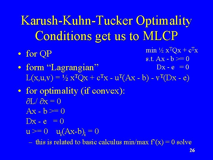
Karush-Kuhn-Tucker Optimality Conditions get us to MLCP • for QP • form “Lagrangian” min ½ x. TQx + c. Tx s. t. Ax - b >= 0 Dx - e = 0 L(x, u, v) = ½ x. TQx + c. Tx - u. T(Ax - b) - v. T(Dx - e) • for optimality (if convex): L/ x = 0 Ax - b >= 0 Dx - e = 0 u >= 0 ui(Ax-b)i = 0 – this is related to basic calculus min/max f’(x) = 0 solve 26

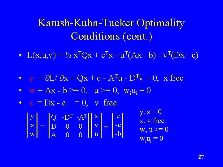
Karush-Kuhn-Tucker Optimality Conditions (cont. ) • L(x, u, v) = ½ x. TQx + c. Tx - u. T(Ax - b) - v. T(Dx - e) • y = L/ x = Qx + c - ATu - DTv = 0, x free • w = Ax - b >= 0, u >= 0, wiui = 0 • s = Dx - e = 0, v free y c Q -DT -AT x s = D 0 0 v + -e w u -b A 0 0 y, s = 0 x, v free w, u >= 0 wiui = 0 27

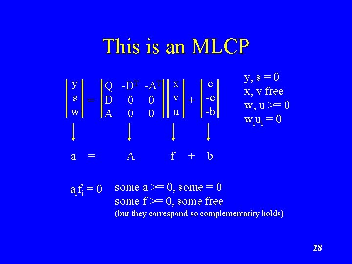
This is an MLCP y c Q -DT -AT x s = D 0 0 v + -e w u -b A 0 0 a = a i fi = 0 A f + y, s = 0 x, v free w, u >= 0 wiui = 0 b some a >= 0, some = 0 some f >= 0, some free (but they correspond so complementarity holds) 28

Modeling Summary • a lot of interesting problems can be formulated as MLCPs – model the problem mathematically – transform it to an MLCP – on paper or in code with wrappers – but what about solving MLCPs? 29

Solving MLCPs (where I hope I made you hungry enough for homework) • Lemke’s Algorithm is only about 2 x as complicated as Gaussian Elimination • Lemke will solve LCPs, which some of these problems transform into • then, doing an “advanced start” to handle the free variables gives you an MLCP solver, which is just a bit more code over plain Lemke’s Algorithm 30

Playing Around With MLCPs • PATH, a MCP solver (superset of MLCP!) • really stoked professional solver • free version for “small” problems • matlab or C • OMatrix (Matlab clone) free trial (omatrix. com) • only LCPs, but Lemke source is in trial » not a great version, but it’s really small (two pages of code) and quite useful for learning, with debug output » good place to test out “advanced starts” • my Lemke’s + advanced start code • not great, but I’m happy to share it • it’s in Objective Caml : ) 31

References for Lemke, etc. • • • free pdf book by Katta Murty on LCPs, etc. free pdf book by Vanderbei on LPs The LCP, Cottle, Pang, Stone Practical Optimization, Fletcher web has tons of material, papers, complete books, etc. • email to authors • relatively new math means authors are still alive, bonus! 32

33

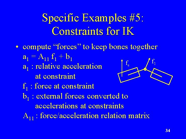
Specific Examples #5: Constraints for IK • compute “forces” to keep bones together a 1 = A 11 f 1 + b 1 fe a 1 : relative acceleration at constraint f 1 : force at constraint b 1 : external forces converted to accelerations at constraints A 11 : force/acceleration relation matrix 34

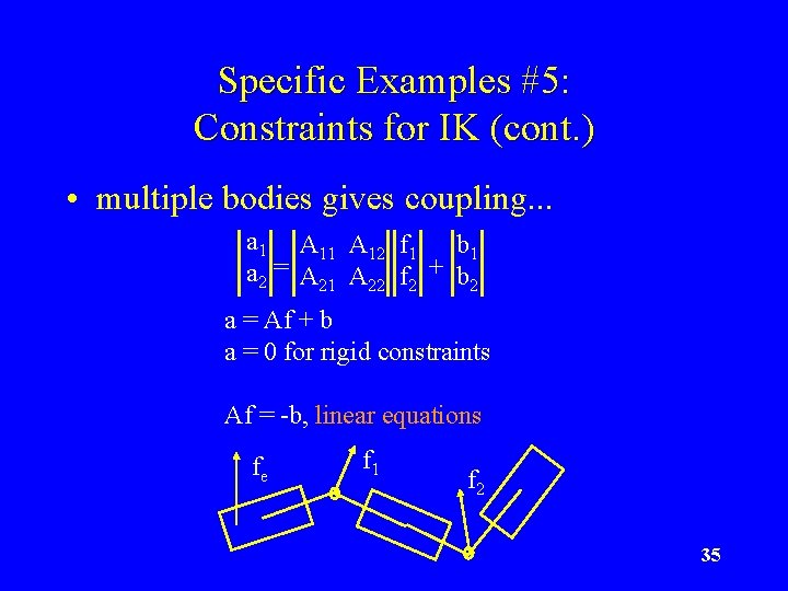
Specific Examples #5: Constraints for IK (cont. ) • multiple bodies gives coupling. . . a 1 A 12 f 1 b 1 a 2 = A 21 A 22 f 2 + b 2 a = Af + b a = 0 for rigid constraints Af = -b, linear equations fe f 1 f 2 35