Lectures on Cellular Automata Continued Modified and upgraded

Lectures on Cellular Automata Continued Modified and upgraded slides of Martijn Schut schut@cs. vu. nl Vrij Universiteit Amsterdam Lubomir Ivanov Department of Computer Science Iona College and anonymous from Internet

Dynamical Systems and Cellular Automata Morphogenetic modeling

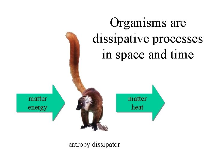
Organisms are dissipative processes in space and time matter energy matter heat entropy dissipator

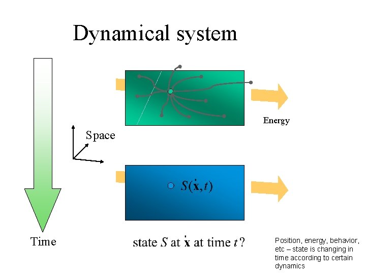
Dynamical system Energy Space Time Position, energy, behavior, etc – state is changing in time according to certain dynamics

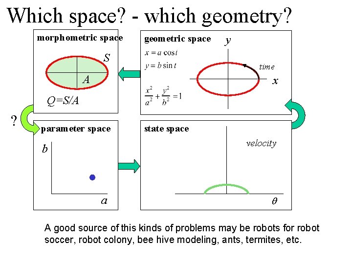
Which space? - which geometry? morphometric space geometric space S y time A x Q=S/A ? parameter space state space velocity b a q A good source of this kinds of problems may be robots for robot soccer, robot colony, bee hive modeling, ants, termites, etc.

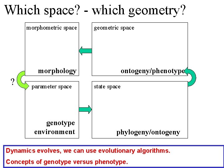
Which space? - which geometry? morphometric space morphology ? parameter space genotype environment geometric space ontogeny/phenotype state space phylogeny/ontogeny Dynamics evolves, we can use evolutionary algorithms. Concepts of genotype versus phenotype.

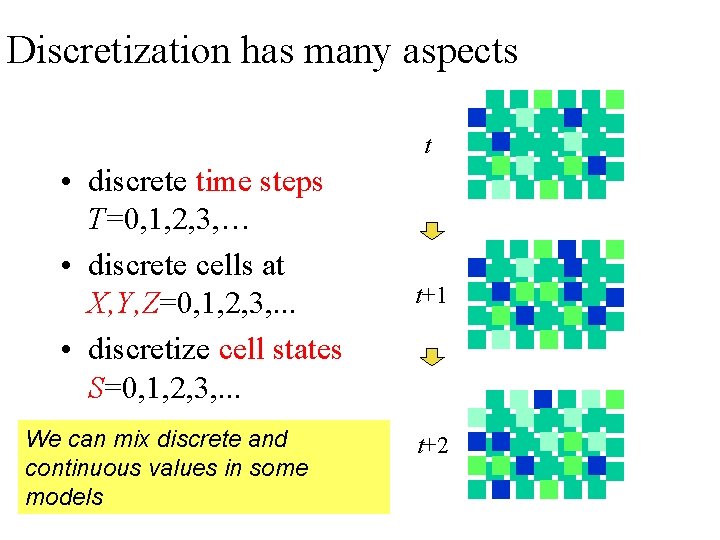
Discretization has many aspects t • discrete time steps T=0, 1, 2, 3, … • discrete cells at X, Y, Z=0, 1, 2, 3, . . . • discretize cell states S=0, 1, 2, 3, . . . We can mix discrete and continuous values in some models t+1 t+2

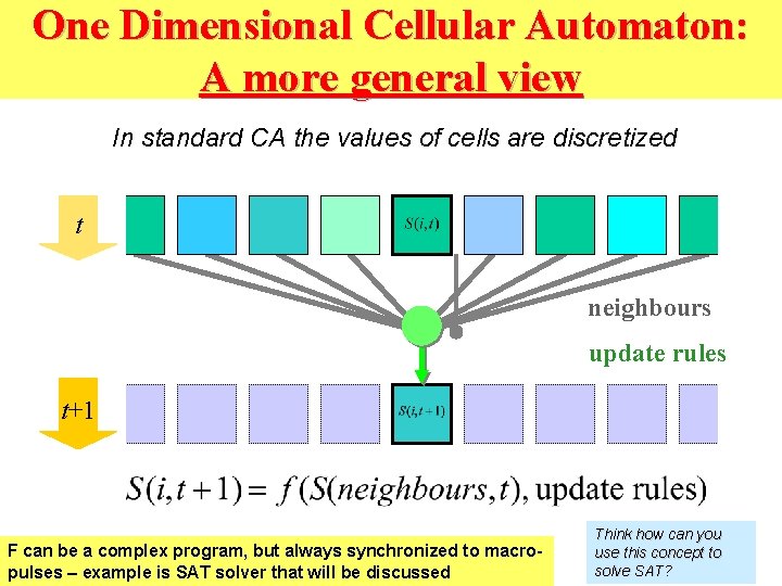
One Dimensional Cellular Automaton: A more general view In standard CA the values of cells are discretized t neighbours update rules t+1 F can be a complex program, but always synchronized to macropulses – example is SAT solver that will be discussed Think how can you use this concept to solve SAT?

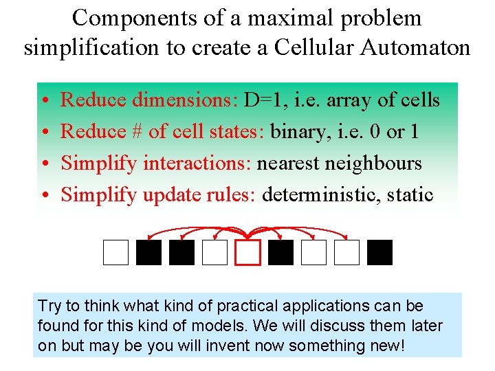
Components of a maximal problem simplification to create a Cellular Automaton • • Reduce dimensions: D=1, i. e. array of cells Reduce # of cell states: binary, i. e. 0 or 1 Simplify interactions: nearest neighbours Simplify update rules: deterministic, static Try to think what kind of practical applications can be found for this kind of models. We will discuss them later on but may be you will invent now something new!

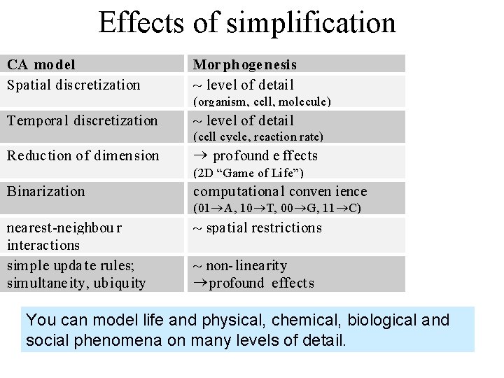
Effects of simplification CA mo del Spatial discretization Mor ph oge nesis ~ level of detail (organism, cell, molecule) Tempora l discretization ~ level of detail (cell cycle, reaction rate) Reduc tion o f dimension pro found e ffects (2 D “Game of Life”) Binarization computationa l conven ience nea rest-neighbou r interactions sim ple upda te rules; sim ultane ity, ub iquity ~ spa tial restrictions (01 A, 10 T, 00 G, 11 C) ~ non- linea rity profound effects You can model life and physical, chemical, biological and social phenomena on many levels of detail.

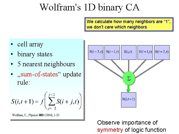
Wolfram's 1 D binary CA We calculate how many neighbors are “ 1”, we don’t care which neighbors • • cell array binary states 5 nearest neighbours „sum-of-states“ update rule: S Wolfram, S. , Physica 10 D (1984), 1 -35 Observe importance of symmetry of logic function

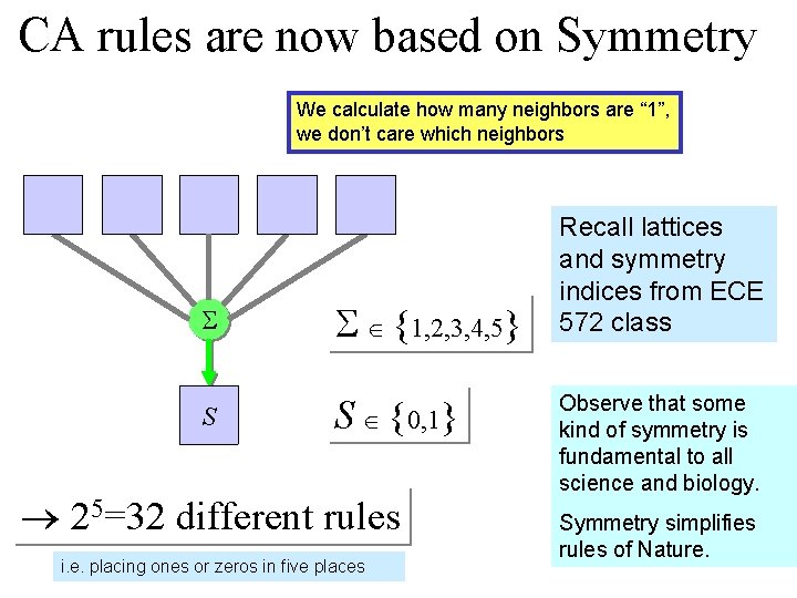
CA rules are now based on Symmetry We calculate how many neighbors are “ 1”, we don’t care which neighbors S S S {1, 2, 3, 4, 5} S {0, 1} 25=32 different rules i. e. placing ones or zeros in five places Recall lattices and symmetry indices from ECE 572 class Observe that some kind of symmetry is fundamental to all science and biology. Symmetry simplifies rules of Nature.

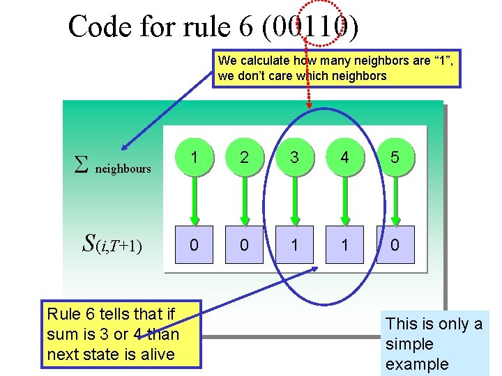
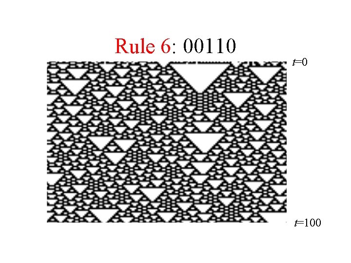
Code for rule 6 (00110) We calculate how many neighbors are “ 1”, we don’t care which neighbors S neighbours 1 2 3 4 5 S(i, T+1) 0 0 1 1 0 Rule 6 tells that if sum is 3 or 4 than next state is alive This is only a simple example

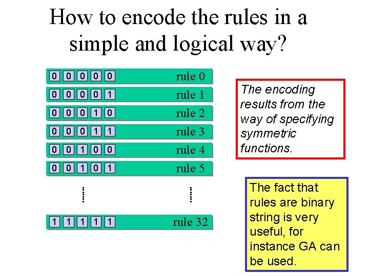
How to encode the rules in a simple and logical way? 0 0 0 0 0 1 1 0 0 0 0 1 1 1 1 rule 0 rule 1 rule 2 rule 3 rule 4 rule 5 rule 32 The encoding results from the way of specifying symmetric functions. The fact that rules are binary string is very useful, for instance GA can be used.

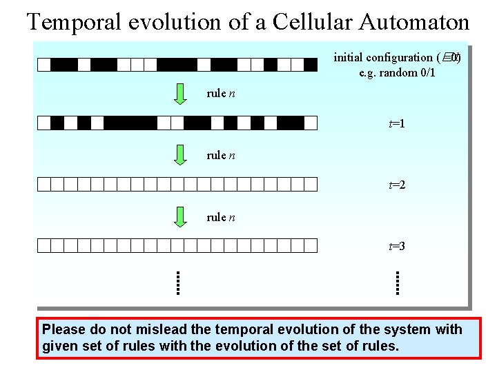
Temporal evolution of a Cellular Automaton initial configuration (�t =0) e. g. random 0/1 rule n t=2 rule n t=3 Please do not mislead the temporal evolution of the system with given set of rules with the evolution of the set of rules.

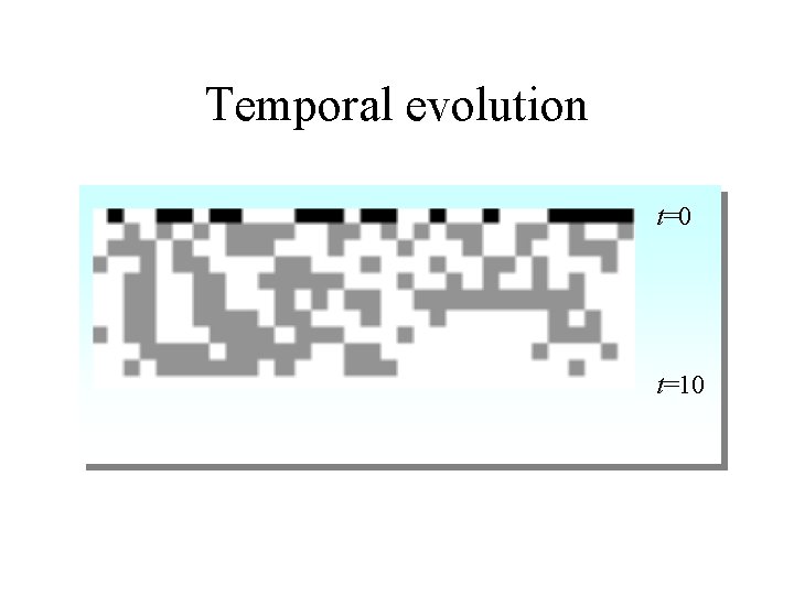
Temporal evolution t=0 t=10

Rule 6: 00110 t=100

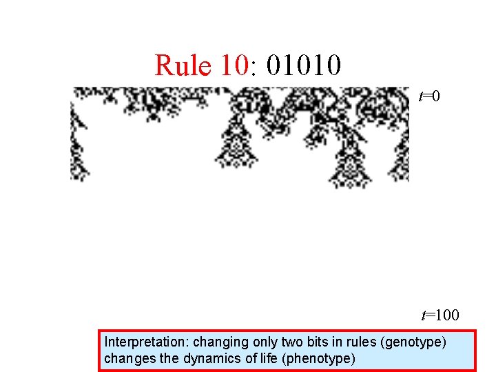
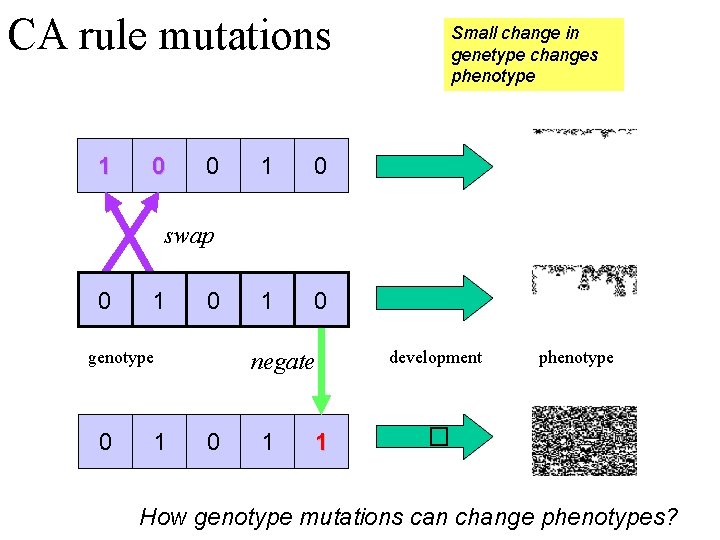
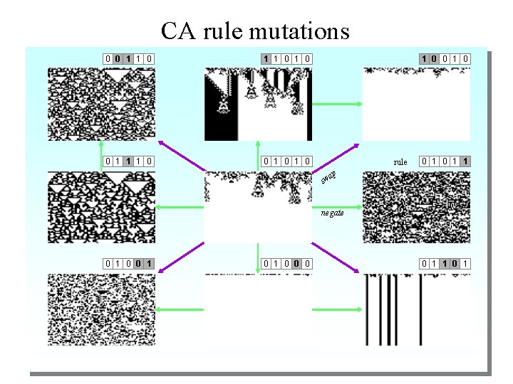
Rule 10: 01010 t=100 Interpretation: changing only two bits in rules (genotype) changes the dynamics of life (phenotype)

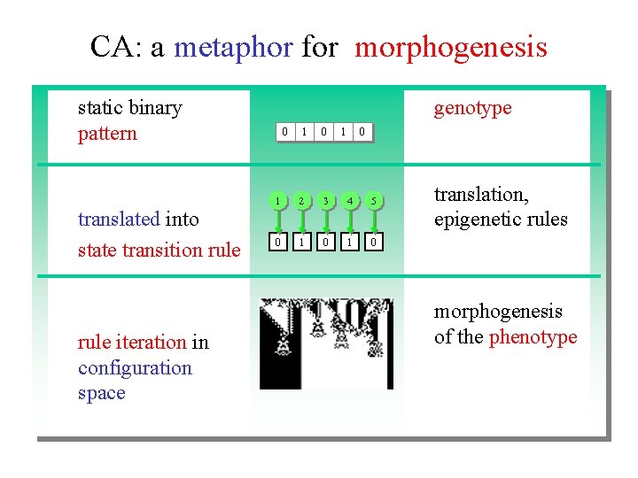
CA: a metaphor for morphogenesis static binary pattern translated into state transition rule iteration in configuration space genotype 0 1 0 1 2 3 4 5 0 1 0 translation, epigenetic rules morphogenesis of the phenotype

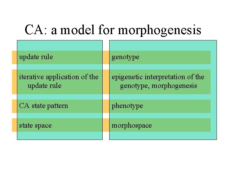
CA: a model for morphogenesis update rule genotype iterative application of the update rule epigenetic interpretation of the genotype, morphogenesis CA state pattern phenotype state space morphospace

CA rule mutations 1 0 0 1 0 Small change in genetype changes phenotype swap 0 1 0 genotype 0 1 negate 0 1 1 development phenotype � How genotype mutations can change phenotypes?

CA rule mutations 0 0 1 1 0 1 0 0 1 1 1 0 0 1 0 1 0 rule 0 1 1 ap sw negate 0 1 0 1 0 0 1 1 0 1

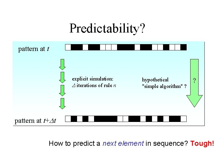
Predictability? pattern at t explicit simulation: D iterations of rule n hypothetical "simple algorithm" ? ? pattern at t+Dt How to predict a next element in sequence? Tough!

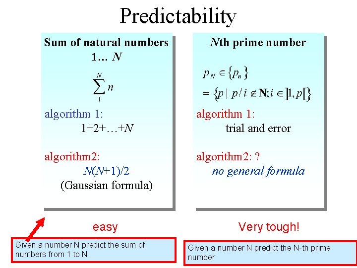
Predictability Sum of natural numbers 1… N Nth prime number algorithm 1: 1+2+…+N algorithm 1: trial and error algorithm 2: N(N+1)/2 (Gaussian formula) algorithm 2: ? no general formula easy Given a number N predict the sum of numbers from 1 to N. Very tough! Given a number N predict the N-th prime number

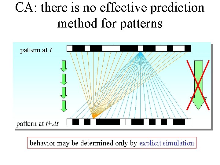
CA: there is no effective prediction method for patterns pattern at t+Dt behavior may be determined only by explicit simulation

CA: deterministic, unpredictable, irreversible • Simple rules generate complex spatio-temporal behavior • For non-trivial rules, the spatio-temporal behaviour is computable but not predictable • The behavior of the system is irreversible • Similarity of rules does not imply similarity of patterns

Aspects of CA morphogenesis • complex relationship between „genotype“ and „phenotype“ • effects of „genes“ are not localizable in specific phenes (pleiotropy) • phenes cannot be traced back to specific single genes (epistasis) epistasis • phenetic effects of "mutations" are not predictable

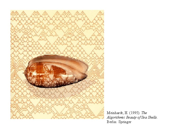
Meinhardt, H. (1995). The Algorithmic Beauty of Sea Shells. Berlin: Springer

Patterns and morphology • Pattern: a spatially and/or temporally ordered distribution of a physical or chemical parameter • Pattern formation • Form (Size and Shape) • Morphogenesis: The spatio-temporal processes by which an organism changes is size (growth) and shape (development)

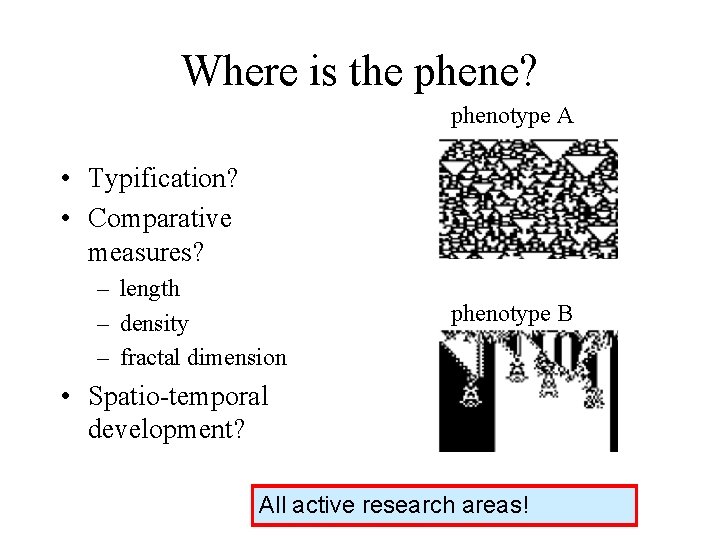
Where is the phene? phenotype A • Typification? • Comparative measures? – length – density – fractal dimension phenotype B • Spatio-temporal development? All active research areas!