Lectures 12 13 Geophysical Inverse Theory I II

Lectures 12 & 13: Geophysical Inverse Theory I, II H. SAIBI & SASAKI Kyushu University Dec. 24, 2015 & Jan. 7, 2016 1

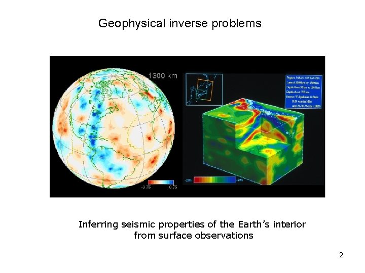
Geophysical inverse problems Inferring seismic properties of the Earth’s interior from surface observations 2

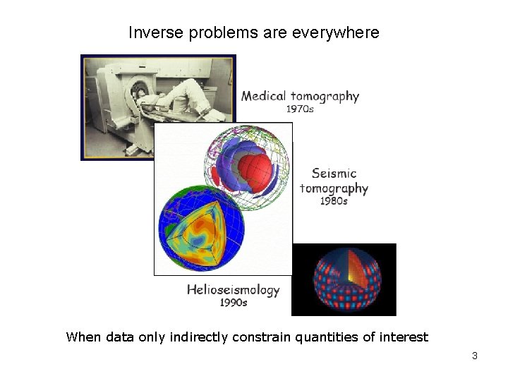
Inverse problems are everywhere When data only indirectly constrain quantities of interest 3

Thinking backwards Most people, if you describe a train of events to them will tell you what the result will be. There are few people, however that if you told them a result, would be able to evolve from their own inner consciousness what the steps were that led to that result. This power is what I mean when I talk of reasoning backward. Sherlock Holmes, A Study in Scarlet, Sir Arthur Conan Doyle (1887) 4

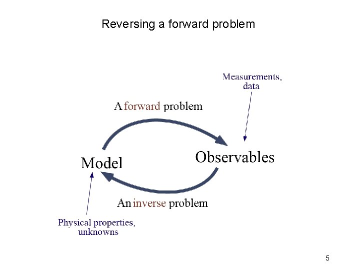
Reversing a forward problem 5

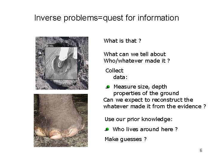
Inverse problems=quest for information What is that ? What can we tell about Who/whatever made it ? Collect data: Measure size, depth properties of the ground Can we expect to reconstruct the whatever made it from the evidence ? Use our prior knowledge: Who lives around here ? Make guesses ? 6

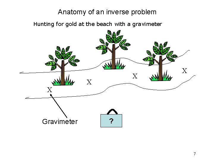
Anatomy of an inverse problem Hunting for gold at the beach with a gravimeter X Gravimeter X X X ? 7

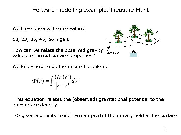
Forward modelling example: Treasure Hunt We have observed some values: 10, 23, 35, 45, 56 gals How can we relate the observed gravity values to the subsurface properties? X Gravimeter X X ? We know how to do the forward problem: This equation relates the (observed) gravitational potential to the subsurface density. -> given a density model we can predict the gravity field at the surface! 8

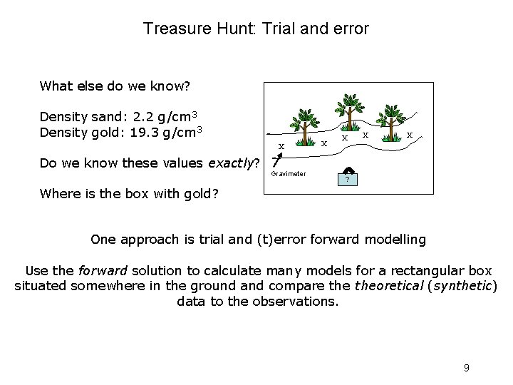
Treasure Hunt: Trial and error What else do we know? Density sand: 2. 2 g/cm 3 Density gold: 19. 3 g/cm 3 X Do we know these values exactly? Gravimeter X X ? Where is the box with gold? One approach is trial and (t)error forward modelling Use the forward solution to calculate many models for a rectangular box situated somewhere in the ground and compare theoretical (synthetic) data to the observations. 9

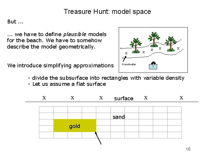
Treasure Hunt: model space But. . . we have to define plausible models for the beach. We have to somehow describe the model geometrically. X X We introduce simplifying approximations Gravimeter X X X ? - divide the subsurface into rectangles with variable density - Let us assume a flat surface x x surface x sand gold 10

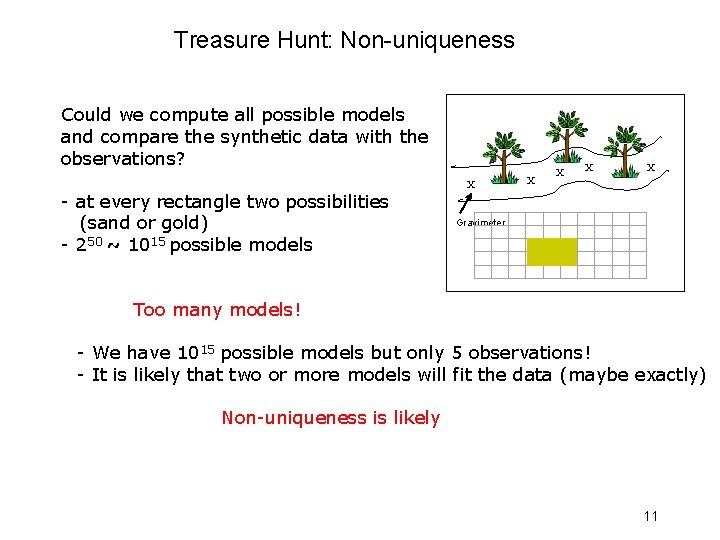
Treasure Hunt: Non-uniqueness Could we compute all possible models and compare the synthetic data with the observations? - at every rectangle two possibilities (sand or gold) - 250 ~ 1015 possible models X Gravimeter X X X Too many models! - We have 1015 possible models but only 5 observations! - It is likely that two or more models will fit the data (maybe exactly) Non-uniqueness is likely 11

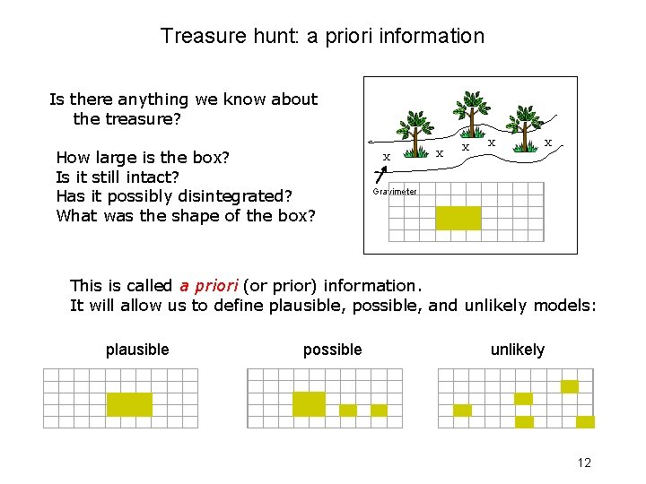
Treasure hunt: a priori information Is there anything we know about the treasure? How large is the box? Is it still intact? Has it possibly disintegrated? What was the shape of the box? X Gravimeter X X X This is called a priori (or prior) information. It will allow us to define plausible, possible, and unlikely models: plausible possible unlikely 12

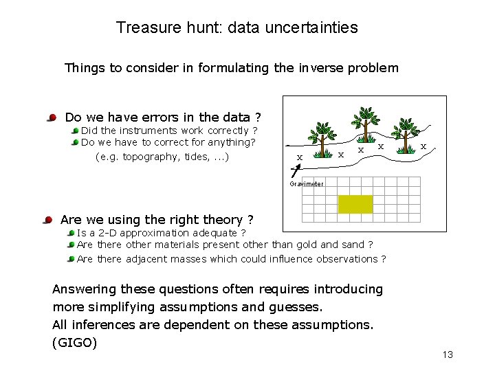
Treasure hunt: data uncertainties Things to consider in formulating the inverse problem Do we have errors in the data ? Did the instruments work correctly ? Do we have to correct for anything? (e. g. topography, tides, . . . ) Are we using the right theory ? X Gravimeter X X X Is a 2 -D approximation adequate ? Are there other materials present other than gold and sand ? Are there adjacent masses which could influence observations ? Answering these questions often requires introducing more simplifying assumptions and guesses. All inferences are dependent on these assumptions. (GIGO) 13

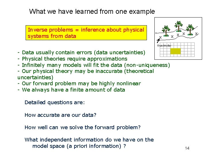
What we have learned from one example Inverse problems = inference about physical systems from data X Gravimeter - Data usually contain errors (data uncertainties) - Physical theories require approximations - Infinitely many models will fit the data (non-uniqueness) - Our physical theory may be inaccurate (theoretical uncertainties) - Our forward problem may be highly nonlinear - We always have a finite amount of data X X X X Detailed questions are: How accurate are our data? How well can we solve the forward problem? What independent information do we have on the model space (a priori information) ? 14

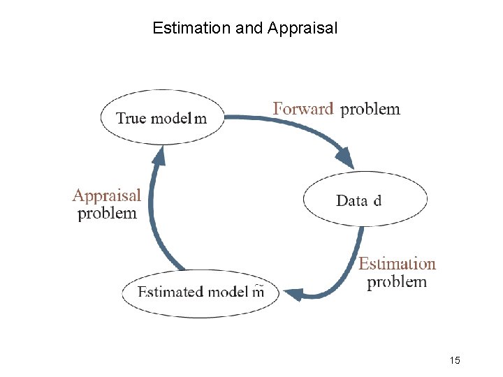
Estimation and Appraisal 15

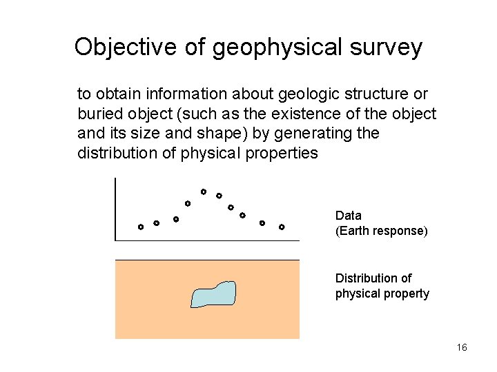
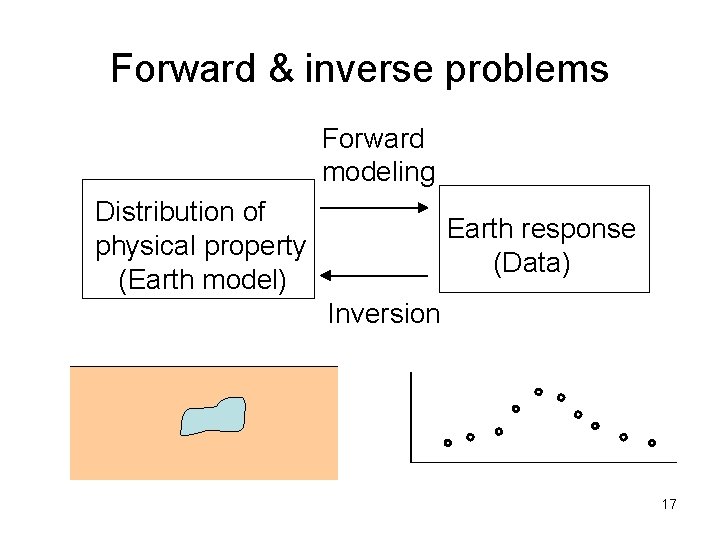
Objective of geophysical survey to obtain information about geologic structure or buried object (such as the existence of the object and its size and shape) by generating the distribution of physical properties Data (Earth response) Distribution of physical property 16

Forward & inverse problems Forward modeling Distribution of physical property (Earth model) Earth response (Data) Inversion 17

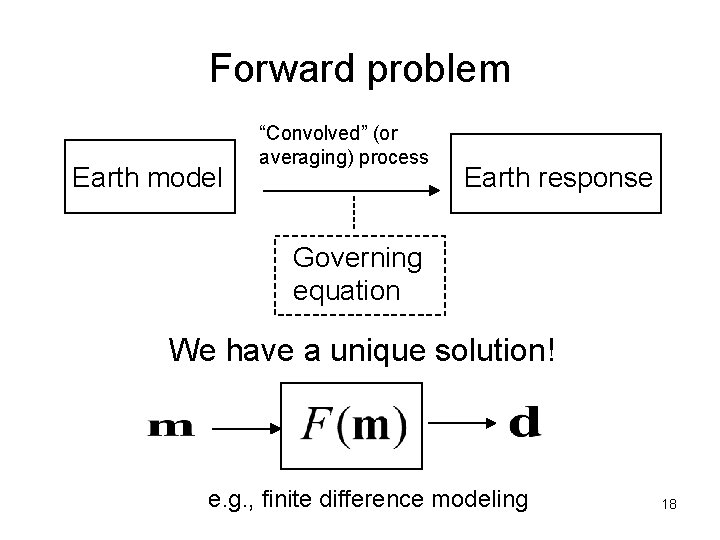
Forward problem Earth model “Convolved” (or averaging) process Earth response Governing equation We have a unique solution! e. g. , finite difference modeling 18

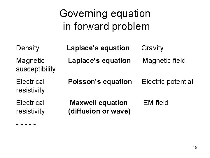
Governing equation in forward problem Density Laplace’s equation Gravity Magnetic susceptibility Laplace’s equation Magnetic field Electrical resistivity Poisson’s equation Electric potential Electrical resistivity Maxwell equation (diffusion or wave) EM field ----19

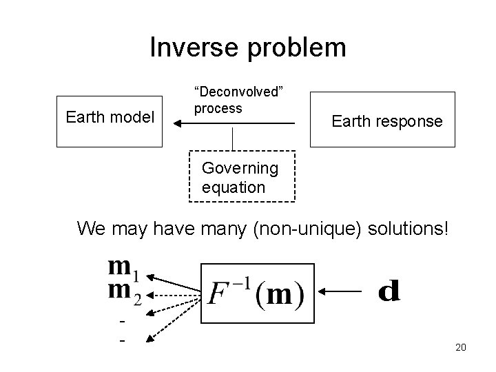
Inverse problem Earth model “Deconvolved” process Earth response Governing equation We may have many (non-unique) solutions! - 20

Why is the inverse solution non-unique? (Why is the inverse problem ill-posed? ) • Data are incomplete; data include measurement errors and various errors. • Data are insufficient; data coverage is limited in space (and in frequency). 21

How to tackle this problem of non-uniqueness Incorporate additional ( a priori) information into the inverse problem Approach to solving the inverse problem as an least-squares problem with constraints (or optimization problem) 22

Regression analysis as an inverse problem In this section, we regard regression analysis as a kind of the inverse problem. Learning regression analysis help to understand the basis of inversion. 23

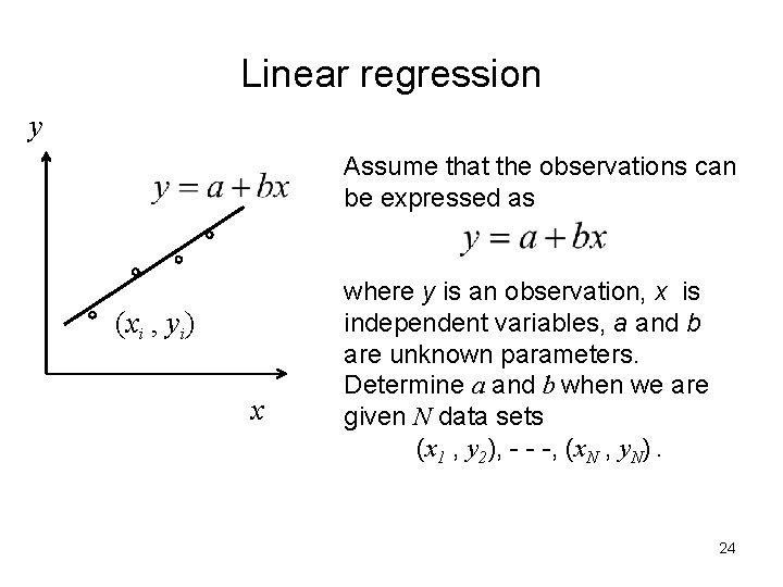
Linear regression y Assume that the observations can be expressed as (xi , yi) x where y is an observation, x is independent variables, a and b are unknown parameters. Determine a and b when we are given N data sets (x 1 , y 2), - - -, (x. N , y. N). 24

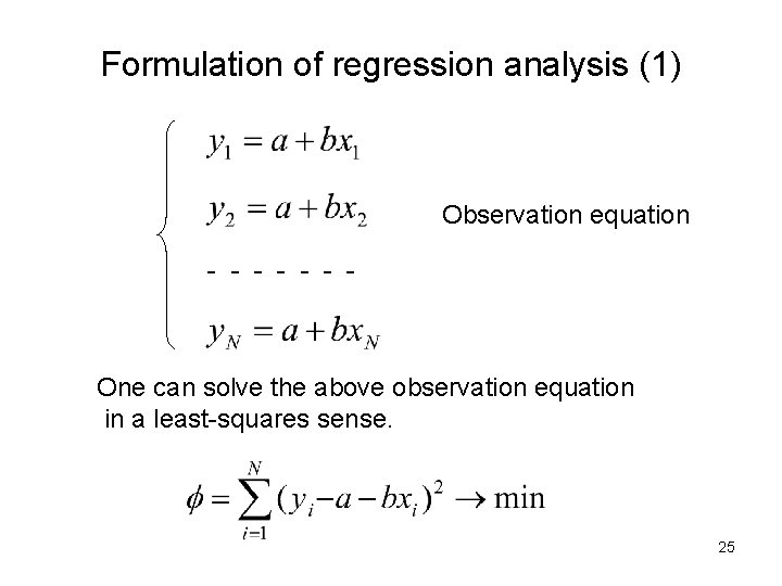
Formulation of regression analysis (1) Observation equation - - - - One can solve the above observation equation in a least-squares sense. 25

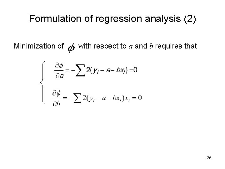
Formulation of regression analysis (2) Minimization of with respect to a and b requires that 26

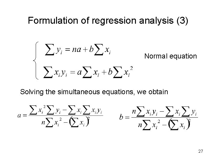
Formulation of regression analysis (3) Normal equation Solving the simultaneous equations, we obtain 27

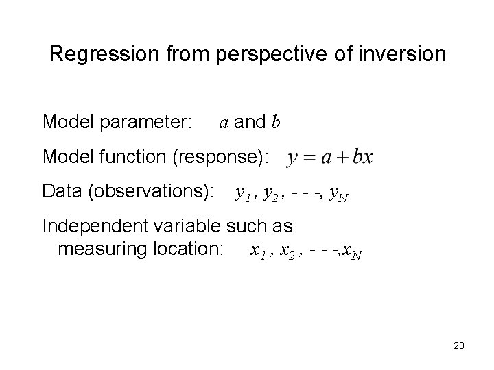
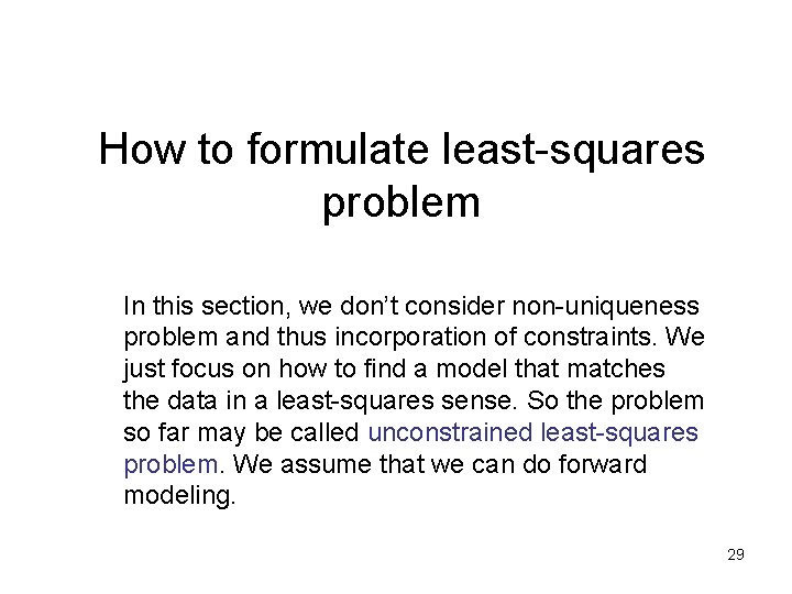
Regression from perspective of inversion Model parameter: a and b Model function (response): Data (observations): y 1 , y 2 , - - -, y. N Independent variable such as measuring location: x 1 , x 2 , - - -, x. N 28

How to formulate least-squares problem In this section, we don’t consider non-uniqueness problem and thus incorporation of constraints. We just focus on how to find a model that matches the data in a least-squares sense. So the problem so far may be called unconstrained least-squares problem. We assume that we can do forward modeling. 29

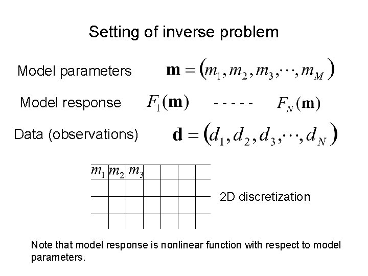
Setting of inverse problem Model parameters Model response ----- Data (observations) 2 D discretization Note that model response is nonlinear function with respect to model parameters.

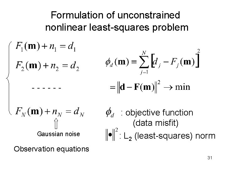
Formulation of unconstrained nonlinear least-squares problem ------ Gaussian noise : objective function (data misfit) : L 2 (least-squares) norm Observation equations 31

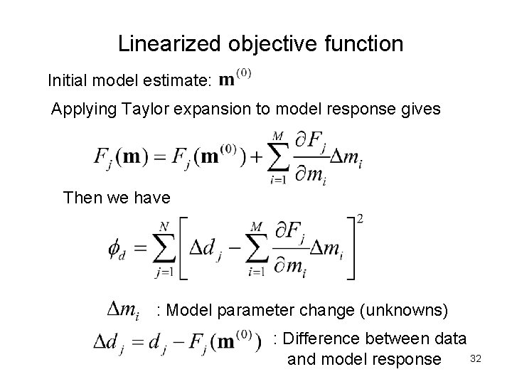
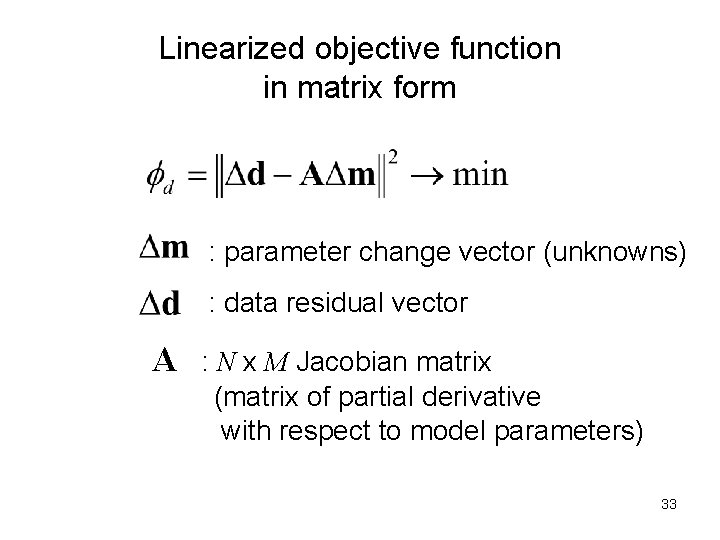
Linearized objective function Initial model estimate: Applying Taylor expansion to model response gives Then we have : Model parameter change (unknowns) : Difference between data 32 and model response

Linearized objective function in matrix form : parameter change vector (unknowns) : data residual vector A : N x M Jacobian matrix (matrix of partial derivative with respect to model parameters) 33

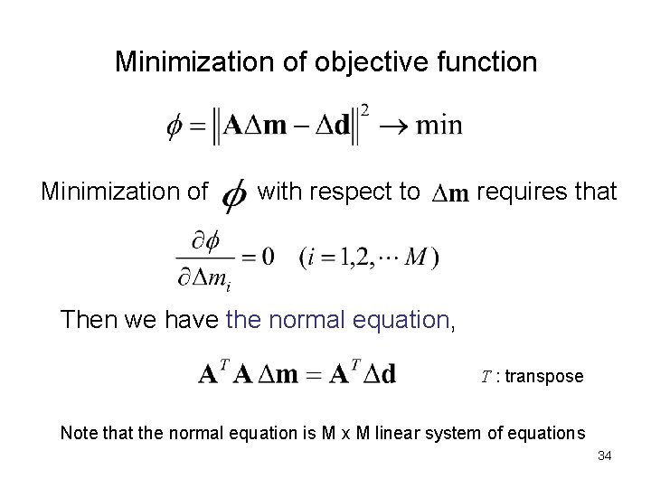
Minimization of objective function Minimization of with respect to requires that Then we have the normal equation, T : transpose Note that the normal equation is M x M linear system of equations 34

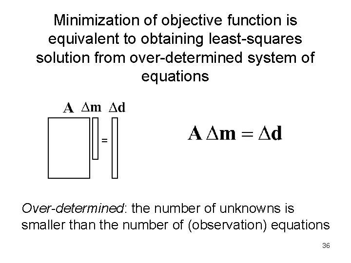
There is an alternative way to obtaining the leastsquares solution by forming the normal equation. It is through forming the over-determined system equations. In general, this approach is more accurate particularly when the number of the unknowns is large. 35

Minimization of objective function is equivalent to obtaining least-squares solution from over-determined system of equations A = Over-determined: the number of unknowns is smaller than the number of (observation) equations 36

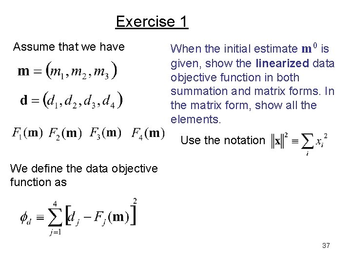
Exercise 1 Assume that we have When the initial estimate m 0 is given, show the linearized data objective function in both summation and matrix forms. In the matrix form, show all the elements. Use the notation We define the data objective function as 37

Exercise 2 Based on the result of Exercise 1, form the over-determined system of equations. 38

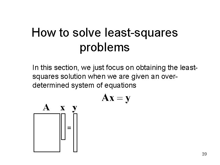
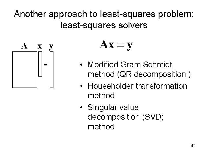
How to solve least-squares problems In this section, we just focus on obtaining the leastsquares solution when we are given an overdetermined system of equations A x y = 39

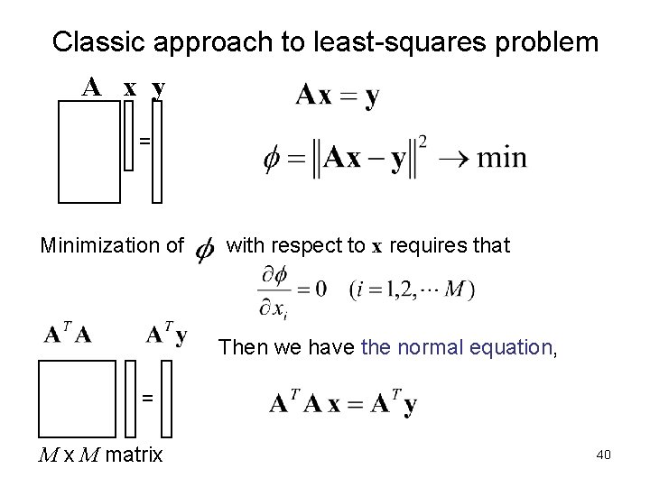
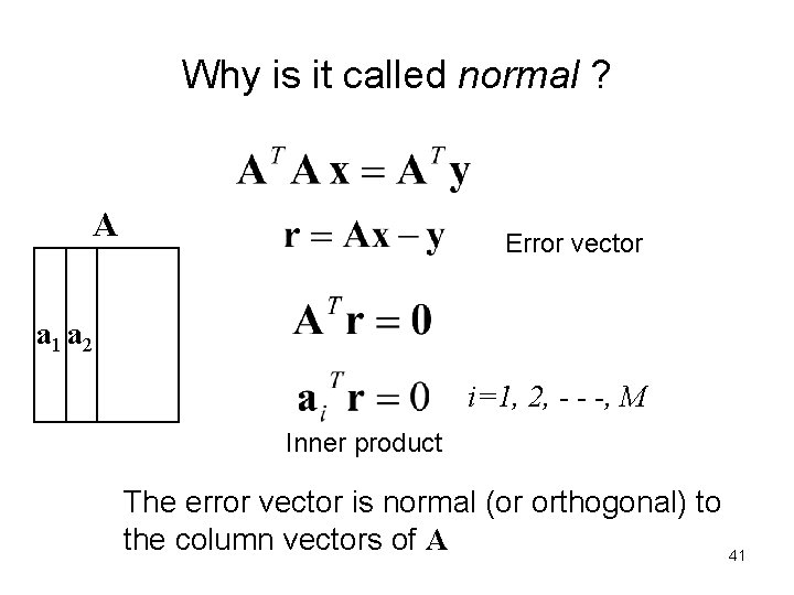
Classic approach to least-squares problem A x y = Minimization of with respect to x requires that Then we have the normal equation, = M x M matrix 40

Why is it called normal ? A Error vector a 1 a 2 i=1, 2, - - -, M Inner product The error vector is normal (or orthogonal) to the column vectors of A 41

Another approach to least-squares problem: least-squares solvers A x y = • Modified Gram Schmidt method (QR decomposition ) • Householder transformation method • Singular value decomposition (SVD) method 42

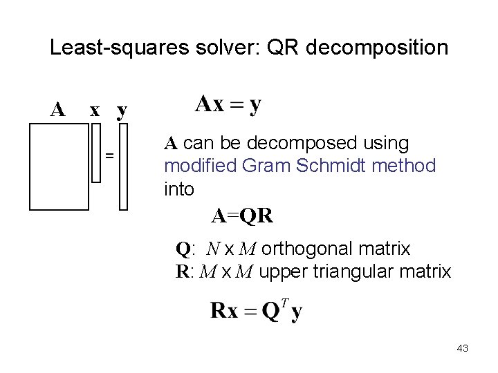
Least-squares solver: QR decomposition A x y = A can be decomposed using modified Gram Schmidt method into A=QR Q: N x M orthogonal matrix R: M x M upper triangular matrix 43

How to incorporate constraints (or a priori information) into a least-squares problem In this section, we consider the most important aspect of inversion, that is, how to pose some soft restrictions on the least-squares solution so that the solution has the likely features of the reality. 44

Prerequisites for solving inverse problems 1) Forward problem can be solved. (Model response can be calculated) 2) Jacobian matrix (or sensitivity matrix) can be obtained 3) Incorporate a priori information (or the likely or expected earth structure) 45

Sidetrack: Occam’s inversion To find the smoothest model so that its features depart from the simplest case only as far as is necessary to fit the data (Constable et al. , 1987) Occam’s razor: 　the explanation of any phenomenon should make as few assumptions as possible, eliminating those that make no difference in the observable predictions of the explanatory hypothesis or theory (Wikipedia). 46

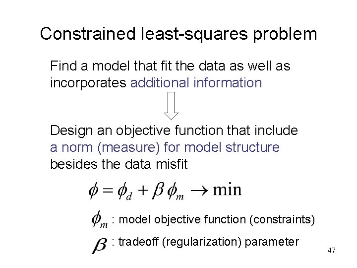
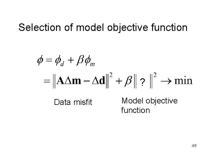
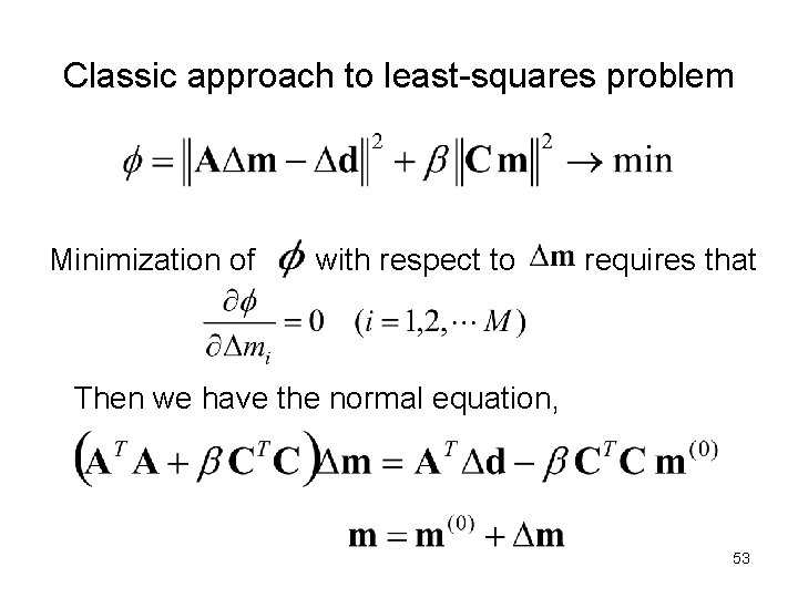
Constrained least-squares problem Find a model that fit the data as well as incorporates additional information Design an objective function that include a norm (measure) for model structure besides the data misfit : model objective function (constraints) : tradeoff (regularization) parameter 47

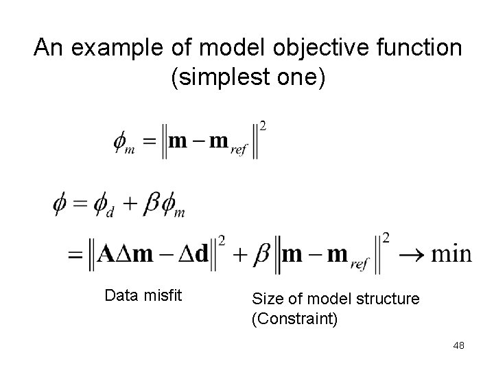
An example of model objective function (simplest one) Data misfit Size of model structure (Constraint) 48

Selection of model objective function ? Data misfit Model objective function 49

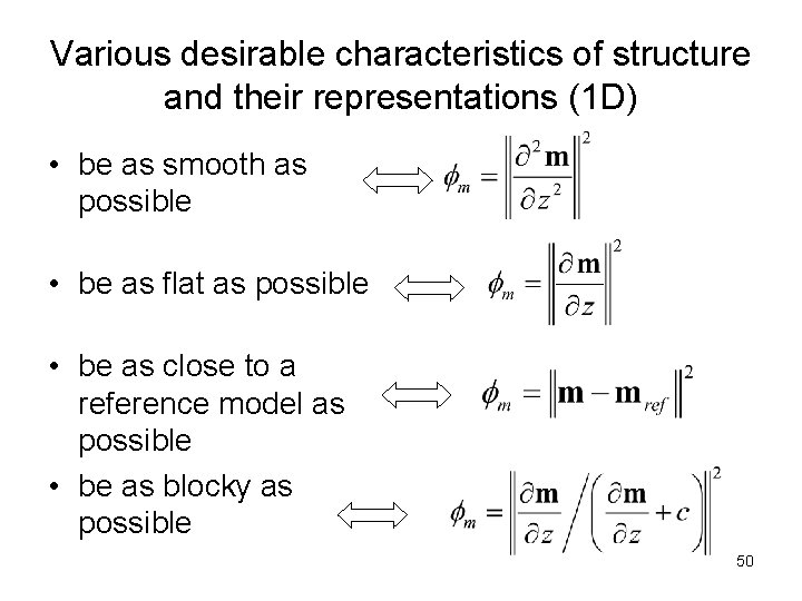
Various desirable characteristics of structure and their representations (1 D) • be as smooth as possible • be as flat as possible • be as close to a reference model as possible • be as blocky as possible 50

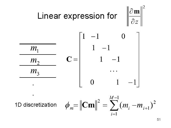
Linear expression for . . 1 D discretization 51

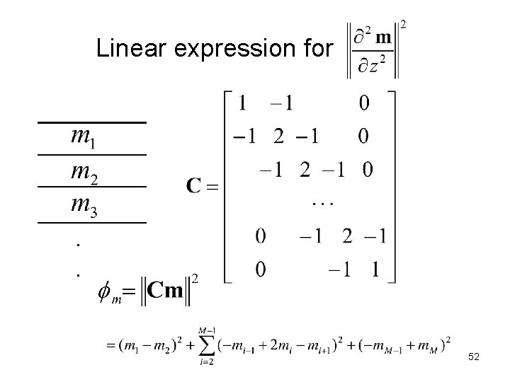
Linear expression for . . 52

Classic approach to least-squares problem Minimization of with respect to requires that Then we have the normal equation, 53

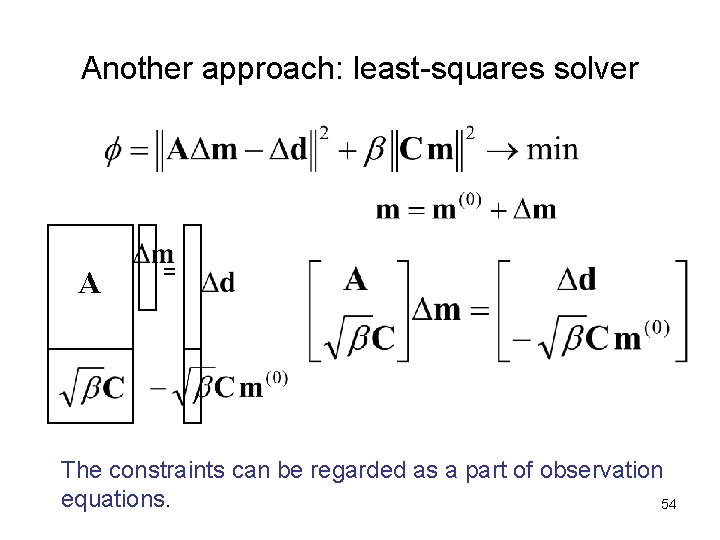
Another approach: least-squares solver A = The constraints can be regarded as a part of observation equations. 54

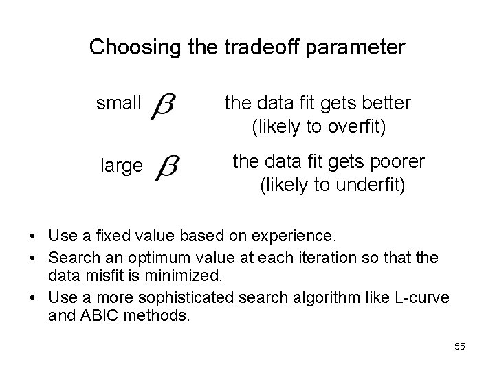
Choosing the tradeoff parameter small large the data fit gets better (likely to overfit) the data fit gets poorer (likely to underfit) • Use a fixed value based on experience. • Search an optimum value at each iteration so that the data misfit is minimized. • Use a more sophisticated search algorithm like L-curve and ABIC methods. 55

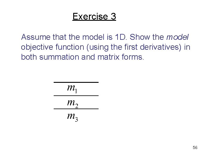
Exercise 3 Assume that the model is 1 D. Show the model objective function (using the first derivatives) in both summation and matrix forms. 56

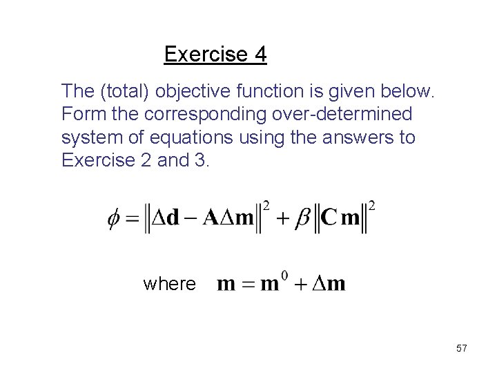
Exercise 4 The (total) objective function is given below. Form the corresponding over-determined system of equations using the answers to Exercise 2 and 3. where 57

Practical tips for evaluating the inversion results You may encounter the results of geophysical inversion as a client of geophysical service companies or you may have to use inversion codes to interpret geophysical data. This section provides practical tips for those cases. 58

In the case of being shown the inversion results Pay attentions to : 1) Data misfit; how well the data fit the model responses. If the data fit is poor, there are two possibilities: the data quality is poor or inversion itself is poor. 2) What kind of a priori information is used. 59

In case of using inversion codes Test the code on the synthetic data for which you have the correct ‘answer’. The simplest way to do this is use the data from homogeneous half-space. For example, for dc resistivity data, you provide 100 ohm-m as the apparent resistivirty data. Start the inversion with the initial model of, say 500 ohm -m and see if the solution converges to the true value of 100 ohm-m. 60

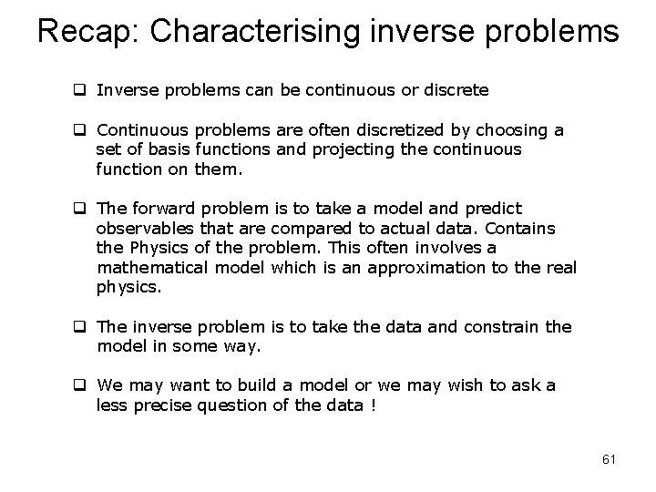
Recap: Characterising inverse problems q Inverse problems can be continuous or discrete q Continuous problems are often discretized by choosing a set of basis functions and projecting the continuous function on them. q The forward problem is to take a model and predict observables that are compared to actual data. Contains the Physics of the problem. This often involves a mathematical model which is an approximation to the real physics. q The inverse problem is to take the data and constrain the model in some way. q We may want to build a model or we may wish to ask a less precise question of the data ! 61

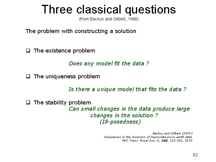
Three classical questions (from Backus and Gilbert, 1968) The problem with constructing a solution q The existence problem Does any model fit the data ? q The uniqueness problem Is there a unique model that fits the data ? q The stability problem Can small changes in the data produce large changes in the solution ? (Ill-posedness) Backus and Gilbert (1970) Uniqueness in the inversion of inaccurate gross earth data. Phil. Trans. Royal Soc. A, 266, 123 -192, 1970. 62

References Oldenburg, D. W. , and Y. Li, 2005, Inversion for applied geophysics: A tutorial, in D. K. Butler, ed. , Near surface geophysics: The society of Exploration Geophysicists, 89 -150. Constable, S. C. , R. L. Parker, and C. G. Constable, 1987, Occam’s Inversion: A practical algorithm for generating smooth models from electromagnetic sounding data, Geophysics, 52, 289 -300. Lines, L. R. , and S. Treitel, 1984, A review on leastsquares inversion and its application to geophysical problems, Geophysical Prospecting, 32, 159 -186. 63

Reference works Understanding inverse theory Ann. Rev. Earth Planet. Sci. , 5, 35 -64, Parker (1977). Interpretation of inaccurate, insufficient and inconsistent data Geophys. J. Roy. astr. Soc. , 28, 97 -109, Jackson (1972). Monte Carlo sampling of solutions to inverse problems J. Geophys. Res. , 100, 12, 431– 12, 447, Mosegaard and Tarantola, (1995) Monte Carlo methods in geophysical inverse problems, Rev. of Geophys. , 40, 3. 1 -3. 29, Sambridge and Mosegaard (2002) 64

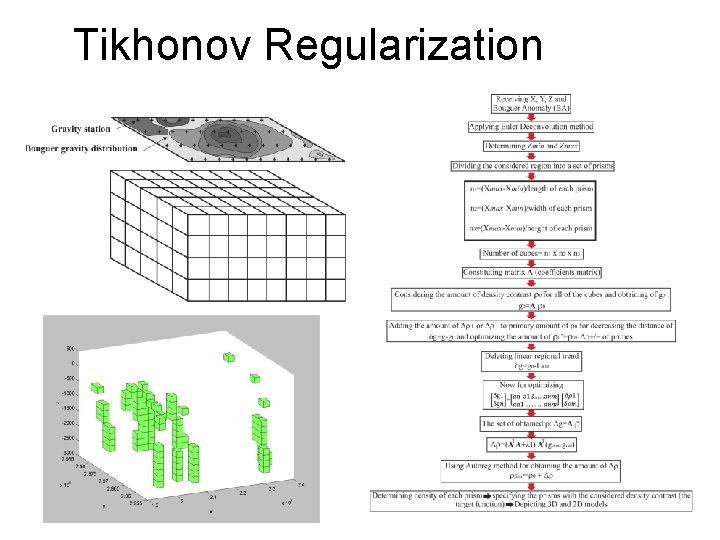
Tikhonov Regularization 65

Lanczos bidiagonalization of gravity 66

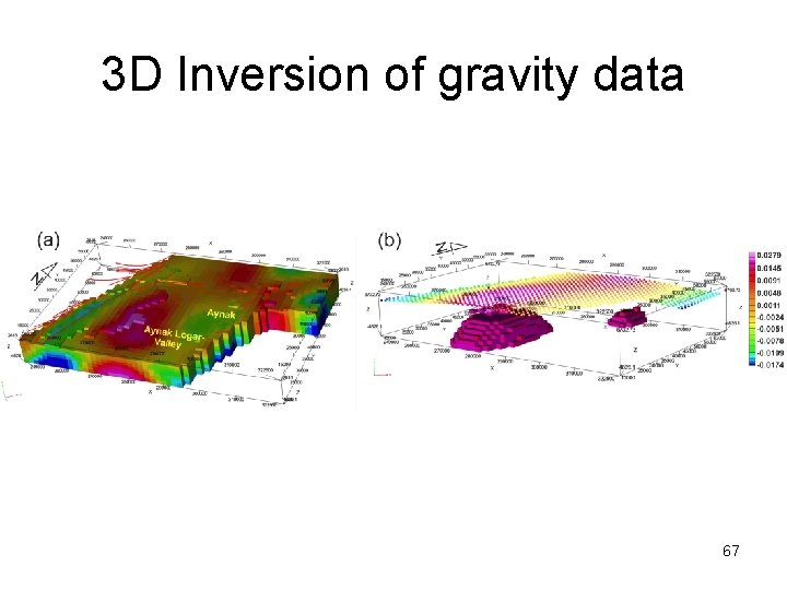
3 D Inversion of gravity data 67

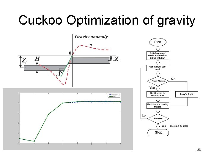
Cuckoo Optimization of gravity 68

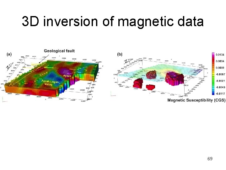
3 D inversion of magnetic data 69

Books See also Menke ‘Geophysical data analysis: discrete inverse theory’ (Academic Press, 1989) 70

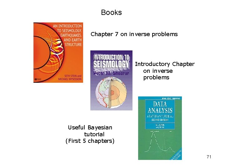
Books Chapter 7 on inverse problems Introductory Chapter on inverse problems Useful Bayesian tutorial (First 5 chapters) 71