LECTURE1 CE 607 STRUCTURAL DYNAMICS SYLLABUS Mid sem25

LECTURE-1 CE 607 STRUCTURAL DYNAMICS

SYLLABUS Mid sem-25 End Exam 60 Free vibration of lumped MDOF system; Approximate methods of obtaining natural frequencies and mode shapes; Frequency domain analysis of MDFS using normal mode theory, Time domain analysis using numerical techniques Principle of virtual works, Modified Rayleigh method, Free and Forced Vibration of continuous structures Refrences: 1. Glen V Berg, elements of structural dynamics, Prentice Hall, NJ W T Thompson, 1983, Theory of vibrations, Prentice hall, New Delhi 2. M Paz, 1984, Structural dynamics, CBS Publishers, New Delhi. 3. J M Biggs, 1964, Introduction to structural dynamics, Mc. Graw-Hill, NY 4. . A K Chopra, 1995, Dynamics of structures, Prentice Hall India, New Delhi

OBJECTIVE: The objective of the course is to understand the behaviour of structure especially building subjected to dynamic loads PRE-REQUISITE: Basic understanding of structural analysis and knowledge of engineering mathematics.

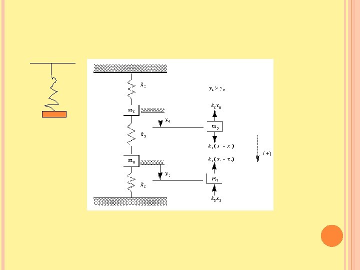
DEGREE OF FREEDOM The minimum number of independent coordinates required to determine completely the positions of all parts of a system at any instant of time defines the degree of freedom of the system. In most cases, we can justifiably discard some components of motion as being insignificant compared with others, thereby get a simplified dynamic system with fewer degree of freedom. A single degree of freedom system requires only one coordinate to describe its position at any instant of time consider a spring mass system.

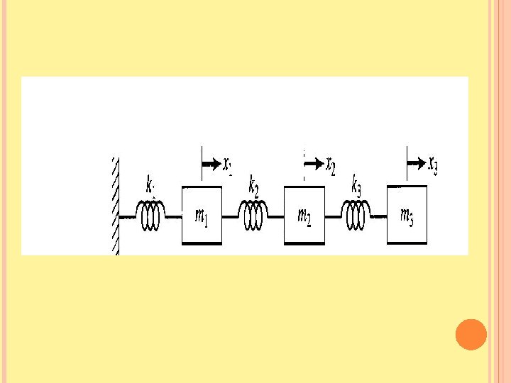
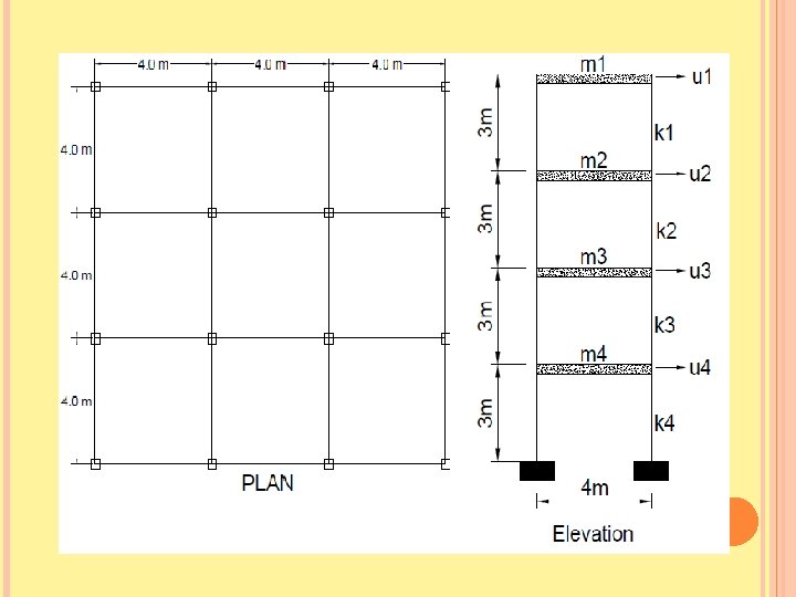
DEGREE OF FREEDOM If Mass of the spring were distributed along its length or if suspended mass is deformable, than there would be infinite degree of freedom But we consider the spring to be weightless, mass to be point mass, and all movements to be in vertical direction so SDF. A more complex case is a three storey plane frame. Mass is distributed so it is continuous system but we idealise the frame as a weightless structural system, with structural components retaining all of their stiffness properties but having no weight, replaced all the mass of the system by three rigid lumped masses attached to the weightless frame at the three floor levels. Then take all motion of lumped mass to be in horizontal direction in the plane of the frame. Then it becomes 3 dof system

IDEALIZATION OF FRAME Let us consider the development of a mathematical model for the lateral load analysis of a ONE storey frame which has 2 nodes, each node has three DOF ie 6 DOF 1. Mass lumped at floor level 2. Infinitely rigid slab/floor 3. No joint rotation 4. No Axial forces

A multi degrees of freedom (dof) system is one, which requires two or more coordinates to describe its motion. For example, for the two story building shown in figure 1 we assume the floor is rigid compared to the two columns. Thus, the displacement of the structure is going to be completely described by the displacement, x, of the floor.

Theoretical procedure of vibration analysis

VIBRATIONS AND CLASSIFICATION OF VIBRATIONS Any motion that repeat itself after an interval of time – vibration or oscillation For a vibration to take place there is a need of application of an external force on elastic bodies such as a spring or a beam or a shaft and then after releasing the force, the body executes a vibratory motion. Vibration can be classified in several ways

TYPES OF VIBRATION In a broader sense vibration is of two types: 1) Free or natural vibration: In free vibration the body at first is given an initial displacement and the force is withdrawn. The body starts vibrating and continues the motion of its own accord. No external force acts on the body further to keep it in motion The frequency of such vibrations depends upon the mass, shape and the elastic properties of the body. It never depends on any external factors. This frequency is called "Free or natural frequency". .

TYPES OF VIBRATION 2)Forced vibration: When a periodic disturbing force keeps the body in vibration through out its entire period of motion, such vibration is said to be a forced vibration. The frequency of vibration of the body is same as the frequency of the applied force.

MULTI DEGREE FREEDOM SYSTEM Systems that require two or more independent coordinates to describe their motion; There are Two masses in the system, it is a 2 DOF system, two equations of motion , one for each mass (more precisely, for each DOF). They are generally in the form of couple differential equation that is, each equation involves all the coordinates.

FREE VIBRATION UNDAMPED CASE

k 1 x 1 k 2(x 2 -x 1) x 1 m 1 k 2(x 1 -x 2) x 2 m 2 Applying Newtons Law m 1 x 1’’ = - k 1 x 1 - k 2 (x 1 - x 2 ) …(1) m 2 x 2’’ = –k 2 (x 2 -x 1) …. (2)

x 2 x 1 k 3 k 2 k 1 m 2

The equations of motion are mx 1' ' = - k(x 1 – x 2). . . . (1) 2 mx 2' ' = - k(x 2 – x 1) - 2 k(x 2 – x 3). . . (2) mx 3'' = - 2 k(x 3 – x 2) = 0. . ……………. . (3)

FREE VIBRATION DAMPED CASE Applying Newtons Law m 1 x 1’’ = - k 1 x 1 - k 2 (x 1 - x 2 ) - c 1 x 1 - c 2 (x 1 - x 2 ) …(1) m 2 x 2’’ = –k 2 (x 2 -x 1) –c 2 (x 2 -x 1) …. (2)

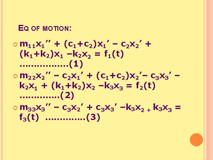
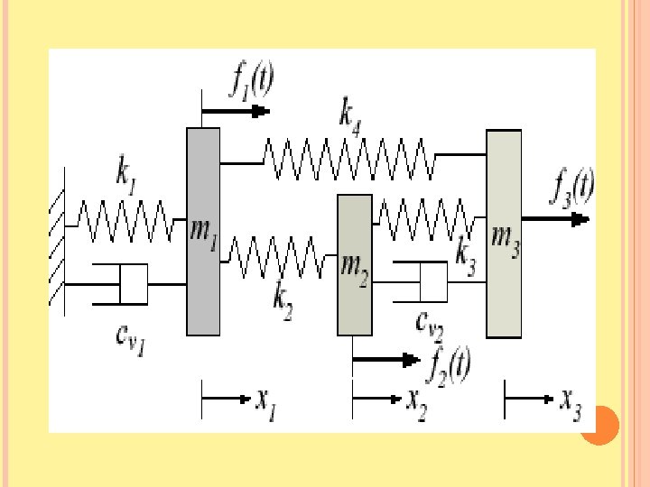
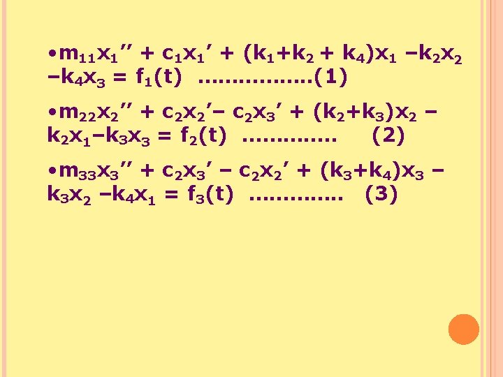
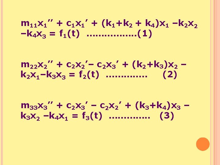
x 1 F 1(t) x 2 F 2(t) m 1 k 1 x 1 m 3 m 2 k 2(x 1 -x 2) c 1 x’ 1 x 3 k 2(x 2 -x 1) k 3(x 3 -x 2) k 4(x 1 -x 3) k 3(x 2 -x 3) m 1 x 1’’ k 4(x 3 -x 1) m 2 x 2’’ m 3 x 3’’

In matrix form the equations become,

The resulting matrix equation of motion is,

Derive the equation of motion for a three degree system lumped mass system. consider the last spring to be non linear where the spring force is given by F 3=k 3 x+k 4 x 2 consider other spring and dampers to be linear

ANALYTICAL SOLUTION FOR FREE VIBRATION UNDAMPED SYSTEM Force = summation of all forces acting ------(1) x 2 x 1 k 2 k 1 m 2

DERIVING EQUATIONS OF MOTION k 1 x 1 k 2(x 1 -x 2) m 1 k 2(x 2 -x 1) m 2 m 1 x 1’’ + k 1 x 1+ k 2(x 1 -x 2)= 0 m 2 x 2’’ + k 2(x 2 -x 1) =0. ……………. . (2) ……………. . (3)

Matrix form of governing equation: where: [M] = mass matrix; [K] = stiffness matrix; Note: Matrices have positive diagonals and are symmetric.

An analytical solution of the MDF equation as it stands is not possible Normal mode concept of vibration is used to recast eq in alternative form Assuming that it is possible to have harmonic motion of m 1 and m 2 at the same frequency ω, we take the solutions as

Assumptions • In free vibration the undamped MDOF system can oscillate in a fixed shape. • The amplitude varies with time. • In free vibration, the displacement vector x(t) can be represented as {x(t)} = {ф}n qn(t)………………(1) Where x(t) is geometrical coordinate; {ф} is a dimensional less constant vector with atleast one nonzero element* ; q is generalized displacement , a function of time. * Nonzero restriction on Φ serves merely to prelude the trival case of no vibration at all.

Eq of motion for an undamped linear system [M]{x’’} + [K]{x} = 0 ………… (2) Put eq 1 ({x(t)} = {ф}n qn(t) ) in eq 2 [M]{ф}n qn(t)’’ + [K]{ф}n qn(t) =0 …. (3) M, K are constants matrices and by hypothesis ф is a constant vector. Thus eq 3 takes the form qn(t)’’ + const qn(t) =0 …. (4) Which is similar to eq of motion for vibration of undamped single degree freedom with constant equal to ωn 2. Thus eq becomes qn(t)’’ + ωn 2 qn(t) =0 …. (5)

Thus eq becomes qn(t)’’ + ωn 2 qn(t) =0 ……. For which the solution is qn(t)=A cos ωn t + B sin ωn t …… (5) (6) If the hypothesis [{x(t)} = {ф}n qn(t)] is valid, then the displacement of the system in free vibration may take the form {x(t)} = {ф}n (A cos ωn t + B sin ωn t)……. (7) Differentiating twice {x’’(t)} =- ωn 2 {ф}n(Acos ωn t + B sin ωn )…. (8

Put eq 7 & 8 in eq 2 {- ωn 2[M] {ф}n + [K] {ф}n } (A cos ωn t + B sin ωn t) =0 …. (9) By hypothesis {ф}n cannot be zero as it is assumed to have one nonzero element. Also A and B should be nonzero. Therfore for soln to exist [ [K] - ωn 2[M]] =0 ………… (10) Thus above singular matrix has zero determinant Ie | [K] - ωn 2[M] | =0

MODAL ORTHOGONALITY Frequency equation for a MDOF system is given as | [K] - ωn 2[M] | {ф}n =0 …………(1) For mode 1 [K] {ф}1 = ω12[M] {ф}1 ……………. (2) PREMULTIPLY BOTH sides of eq 2 by {ф} 2 T[K] {ф}1 ……. (3) = ω12 {ф} 2 T[M] {ф}1

Similarly for mode 2 [K] {ф}2 = ω22[M] {ф}2 ……………. (4) PREMULTIPLY BOTH sides of eq 4 by {ф}1 T[K] {ф}2 ……. (5) = ω22 {ф}1 T[M] {ф}2 Transposing LHS and RHS of eq 3 ie [{ф} 2 T[K] {ф}1]T [{ф} 2 [K] T{ф}1 T …. (6) = = [ω12 {ф} 2 T[M] {ф}1 ]T ω12 {ф} 2 [M]T {ф}1 T

Since [K] and [M] are symetrical so [K] T=[K] and[M]T = [M] therefore Eq 6 may be written as [{ф} 2 [K]{ф}1 T …. (7) = ω12 {ф} 2 [M] {ф}1 T Subtracting 7 from 5 ω22 {ф}1 T[M] {ф}2 - ω12 {ф} 2 [M] {ф}1 T = 0…(8) or ( ω22 - ω12 ){ф} 2 [M] {ф}1 T = 0 …(9)

ω2 ‡ ω1, so {ф}1 T [M] {ф} 2 = 0 …………. . Put eq 10 in 7 {ф}1 T [K] {ф} 2 = 0 ……………. . (10) (11) Eq 10 and eq 11 are the orthogonality relations for mode 1 and 2. In general for p not equal to r {ф}p. T [M] {ф}r = 0 …………. . (12) and {ф}p. T [K] {ф}r = 0 …………. . (13)

THIS IS CALLED ORTHOGINALITY PRINCIPLE. EIGEN VECTORS ARE UNIQUE. AN SCALAR MULTIPLIER OF AN EIGEN VECTOR IS ALSO SCALAR. {Ф} RT [M] {Ф} R = SCALAR IF SCALAR IS 1 , IT IS CALLED NORMAL MODE.

The orthogonality of natural frequencies implies that the following square matrix are diagonal: {ф}r. T [M] {ф}r =[M] …………. . (14) and {ф}r. T [K] {ф}r = [K] …………. . (15)

which represent two simultaneous homogenous algebraic equations in the unknown X 1 and X 2. For trivial solution, i. e. , X 1 = X 2 = 0, there is no solution. For a nontrivial solution, the determinant of the coefficients of X 1 and X 2 must be zero: or

FREE VIBRATION ANALYSIS OF AN UNDAMPED SYSTEM which is called the frequency or characteristic equation. Hence the roots are: The roots are called natural frequencies of the system.

FREE VIBRATION ANALYSIS OF AN UNDAMPED SYSTEM To determine the values of X 1 and X 2, given ratio The normal modes of vibration corresponding to ω12 and ω22 can be expressed, respectively, as which are known as the modal vectors of the system. 47

FREE VIBRATION ANALYSIS OF AN UNDAMPED SYSTEM The free vibration solution or the motion in time can be expressed itself as Where the constants , , and are determined by the initial conditions. The initial conditions are 48

SPECIAL CASE Let m 1=m 2=m and k 1=k 2=k 3=k. Then:

SOLUTION OF EQUATIONS OF MOTION We know from experience that: Substituting the above equation to eq. of motion, we obtain two eqs w. r. t. X 1, X 2 : The above two equations are satisfied for every t

Trivial solution A, B=0. In order to have a nontrivial solution: First natural frequency: The displacement for the first natural frequency is: This vector is called mode shape. Constant cannot be determined. Usually assume first entry is 1. Therefore, mode shape is:

Thus, both masses move in phase and the have the same amplitudes.

Second natural frequency: Mode shape for above frequency: Usually assume first entry is 1. Therefore, mode shape is: The two masses move in opposite directions.

Displacements of two masses are sums of displacements in the two modes:

OBSERVATIONS: System motion is superposition of two harmonic (sinusoidal) motions with frequencies 1 and 2. Participation of each mode depends on initial conditions. Four unknowns (c 1, c 2, 1, 2) can be found using four initial conditions. Can find specific initial conditions so that only one mode is excited.

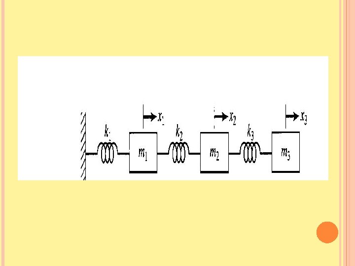
The equations of motion are m 1 x 1' ' = - k 1 x 1 – k 2(x 1 – x 2). . . . (1) m 2 x 2' ' = - k 2(x 2 – x 1) - k 3(x 2 – x 3). . . (2) m 3 x 3'' = - k 3(x 3 – x 2). . ……………. . (3)

Find frequency and mode shape for 0

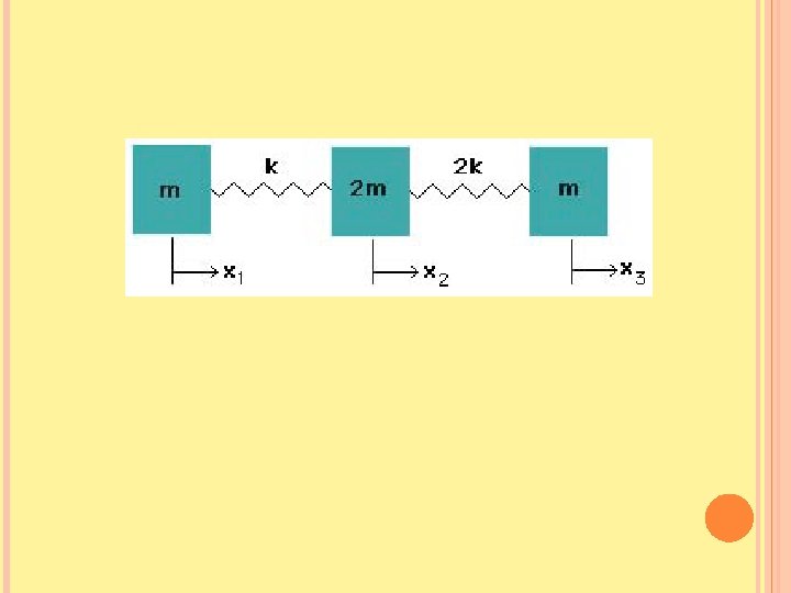
DERIVING EQUATIONS OF MOTION 2 mx 1’’ 2 kx 1 k(x 1 -x 2) 2 m m k(x 2 -x 1) 2 mx 1’’ = – 2 kx 1 - k(x 1 -x 2) mx 2’’ = -k(x 2 -x 1) ……………. . (2) Rearranging 2 mx 1“ + 3 kx 1 -kx 2 =0 ------ (3) mx“ - kx 1+ kx 2 =0 ------ mx 2’’ (4)

Assuming that it is possible to have harmonic motion of 2 m and m at the same frequency ω, we take the solutions as

Substituting into Eqs. (3) and (4), Since Eq. (7) must be satisfied for all values of the time t, the terms between brackets must be zero. Thus, The characteristic equation from the determinant of the above matrix is | [K] - ωn 2[M] | =0 -----(9)

Where [M] = 2 m 0 [K] = 2 k+k -k 0 m -k k

Substitute values in frequency eq | [K] - ωn 2[M] | =0 2 k+k -k Or 3 k – 2 m ωn 2 -k -k k – m ωn 2 Or 3 k 2 -3 km ωn 2 -2 km 2 ωn 2 +2 mk ωn 4 – k 2=0 Or 2 m 2 k ωn 4 +3 k 2 -3 km ωn 2 -2 km ωn 2 +2 k 2=0 Or ωn 4 –(5 k/2 m)ωn 2 + k 2/m 2=0 Solve for ωn 2 -k k - ωn 2 2 m 0 0 =0 m =0

ωn 2 =k/2 m[5/2 +-3/2] Or ωn 2 = 2 k/m and ωn 2 =k/2 m Finally ω1 = SQRT( k/2 m) ω2 = SQRT(2 k/m) Put value of k ie 24 EI/h 3 ω1 = 3. 464 SQRT(EI/mh 3) ω2 = 6. 928 SQRT(EI/mh 3)

MODE SHAPES 2 K +K -K -K X 1 K X 2 - ΩN 2 2 M 0 0 M 3 k. X 1 –k. X 2 – 2 m ωn 2 X 1 =0 -k. X 1 + k. X 2 – m ωn 2 X 2 =0 X 1 = 0 X 2 0

X 1/X 2 = k/(3 k-2 m ωn 2 ) Or Put ω12 X 1/X 2 = k/2 k =1/2 (first mode shape) Put ω22 X 1/X 2 = k/2 k =1/-1 (second mode shape)

Derive the equation of motion for a three degree system lumped mass system shown below. also Find frequency and mode shapes for the system assuming m 1=m 2=m 3=m and k 1=k 2=k 3=k 4=k 5=k 6=k

DAMPED FREE FIBRATION Applying Newtons Law m 1 x 1’’ = - k 1 x 1 - k 2 (x 1 - x 2 ) - c 1 x 1 - c 2 (x 1 - x 2 ) …(1) m 2 x 2’’ = –k 2 (x 2 -x 1) –c 2 (x 2 -x 1) …. (2) MX” + CX’ +KX=0

Derive the equation of motion for a three degree system lumped mass system. consider the last spring to be non linear where the spring force is given by F 3=k 3 x+k 4 x 2 consider other spring and dampers to be linear

FORCED VIBRATION

EQUATION OF MOTION FORCED VIBRATION Consider a viscously damped two degree of freedom spring-mass system, shown in Fig.

EQUATIONS OF MOTION FORCED VIBRATION 71 The application of Newton’s second law of motion to each of the masses gives the equations of motion: Both equations can be written in matrix form as where [m], [c], and [k] are called the mass, damping, and stiffness matrices, respectively, and are given by

EQUATIONS OF MOTION FORCED VIBRATION 72 And the displacement and force vectors are given respectively: It can be seen that the matrices [m], [c], and [k] are all 2 x 2 matrices whose elements are known masses, damping coefficient and stiffnesses of the system, respectively.

EQUATIONS OF MOTION FORCED VIBRATION o. Further, these matrices can be seen to be symmetric, so that, where the superscript T denotes the transpose of the matrix. o. The solution of Eqs. (1) and (2) involves four constants of integration (two for each equation). Usually the initial displacements and velocities of the two masses are specified as x 1(t = 0) = x 1(0) and x 2(t = 0) = x 2(0) and 1( t = 0) = 2 (t = 0) = 1(0), 2(0). 73

Derive the equation of motion for a three degree system lumped mass system shown below

In matrix form the equations become,

The resulting matrix equation of motion is,