Lecture Three Chapters Two and three Photo slides
- Slides: 33

Lecture Three Chapters Two and three Photo slides from Digital Image Processing, Gonzalez and Woods, Copyright 2002

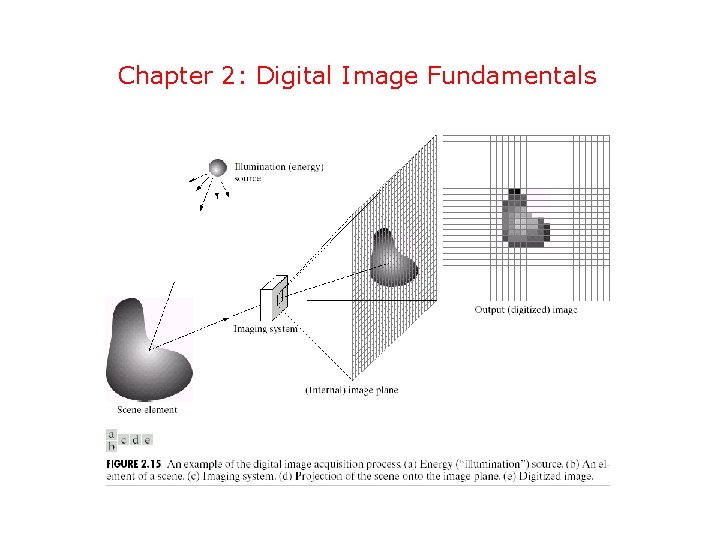
Chapter 2: Digital Image Fundamentals

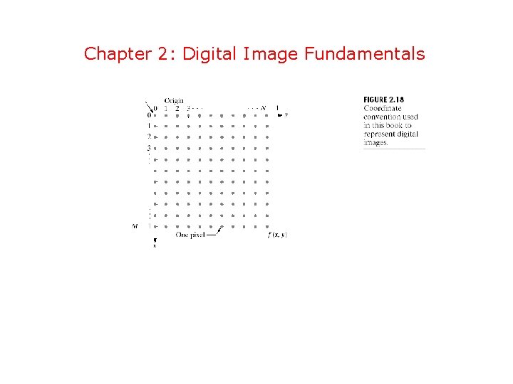
Functional Represenation of Images • Two-D function f(x, y), (x, y) pixel position. Postive and bounded • Written as f(x, y)=i(x, y)r(x, y), i(x, y) illumination from light source, r(x, y) reflectance (bounded between 0 and 1) based on material properties. E. g r(x, y)=0. 01 for black velvet, r(x, y) = 0. 93 for snow. • Intensity of monochrome image f(x, y) is synonymous with grey levels. By convention grey level are from 0 to L 1.

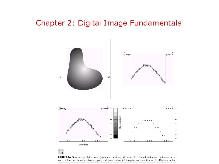
Chapter 2: Digital Image Fundamentals

Chapter 2: Digital Image Fundamentals

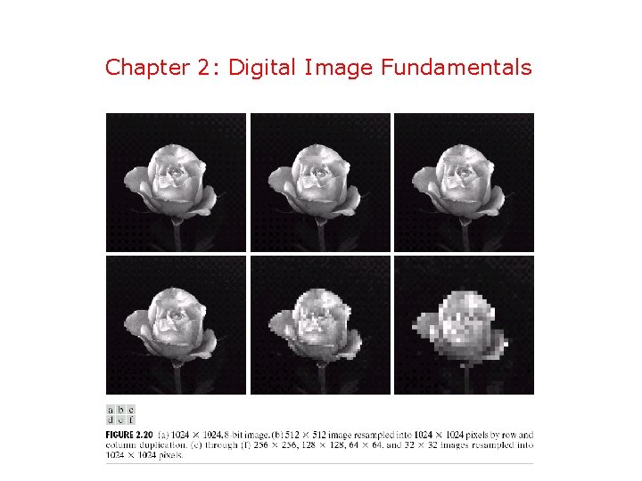
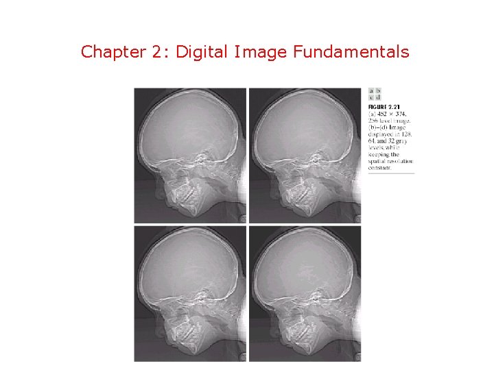
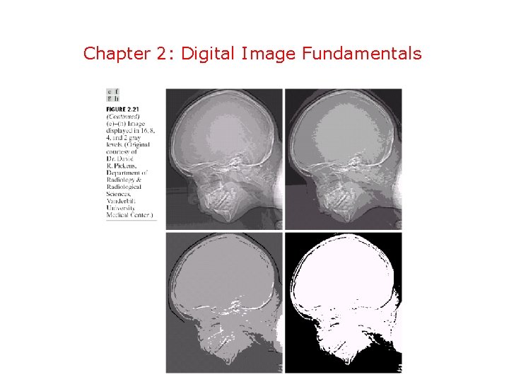
Spatial and Gray Level Resolution • Spatial resolution is the smallest level of detail discernable in an image. Number of line pairs per millimeter, say 100 line pairs per millimeter. • Gray-level resolution is the smallest discernable change in gray level. Very subjective.

Chapter 2: Digital Image Fundamentals

Chapter 2: Digital Image Fundamentals

Chapter 2: Digital Image Fundamentals

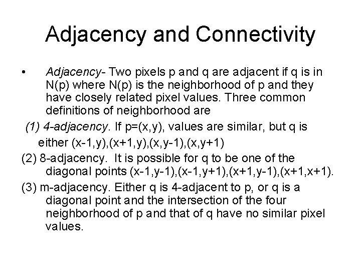
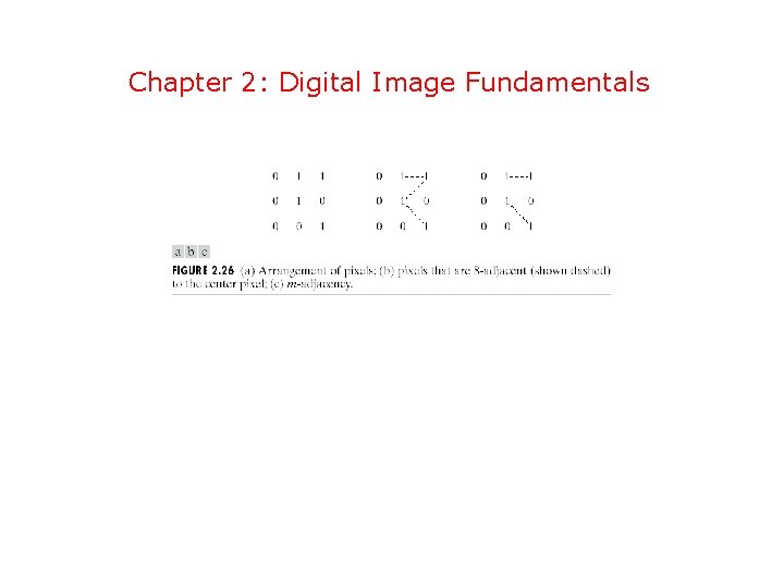
Adjacency and Connectivity • Adjacency- Two pixels p and q are adjacent if q is in N(p) where N(p) is the neighborhood of p and they have closely related pixel values. Three common definitions of neighborhood are (1) 4 -adjacency. If p=(x, y), values are similar, but q is either (x-1, y), (x+1, y), (x, y-1), (x, y+1) (2) 8 -adjacency. It is possible for q to be one of the diagonal points (x-1, y-1), (x-1, y+1), (x+1, y-1), (x+1, x+1). (3) m-adjacency. Either q is 4 -adjacent to p, or q is a diagonal point and the intersection of the four neighborhood of p and that of q have no similar pixel values.

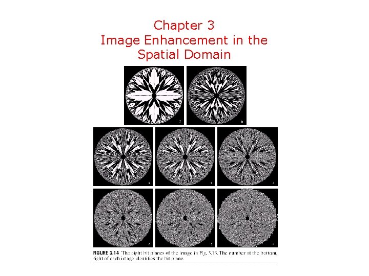
Chapter 3 Image Enhancement in the Spatial Domain

Chapter 2: Digital Image Fundamentals

Adjacency , More Formally Choose a set of gray values V. If f(p) and f(q) are in V, and q is in the right kind of neighborhood of p, then p and q are adjacent. I can model this relationship using 0 -1 images, why? ?

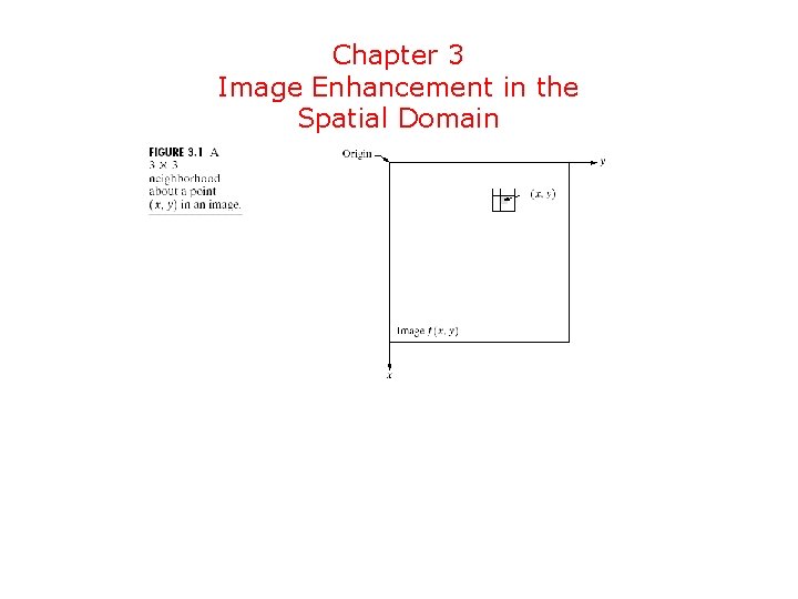
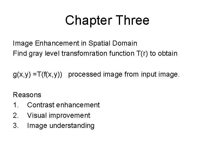
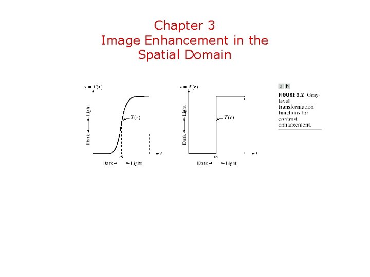
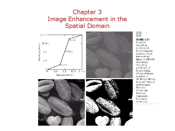
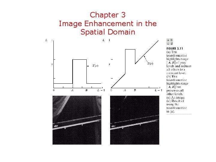
Chapter Three Image Enhancement in Spatial Domain Find gray level transfomration function T(r) to obtain g(x, y) =T(f(x, y)) processed image from input image. Reasons 1. Contrast enhancement 2. Visual improvement 3. Image understanding

Chapter 3 Image Enhancement in the Spatial Domain

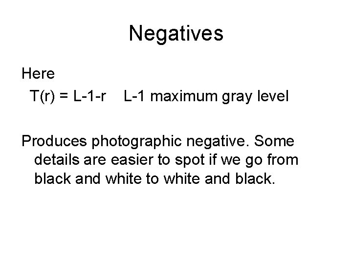
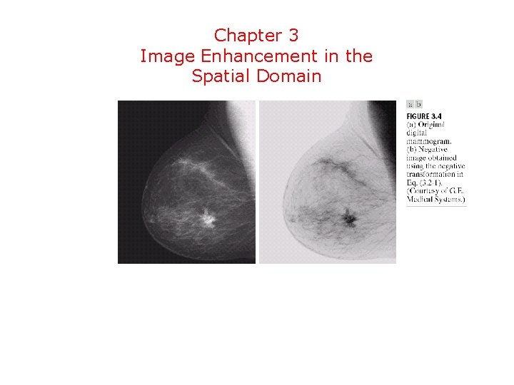
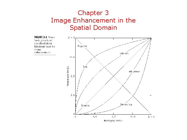
Negatives Here T(r) = L-1 -r L-1 maximum gray level Produces photographic negative. Some details are easier to spot if we go from black and white to white and black.

Chapter 3 Image Enhancement in the Spatial Domain

Mammogram Notice that the white or gray detail in the dark region is more visible in the negative. This shows a small lesion.

Chapter 3 Image Enhancement in the Spatial Domain

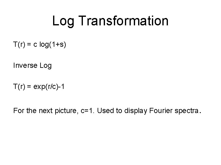
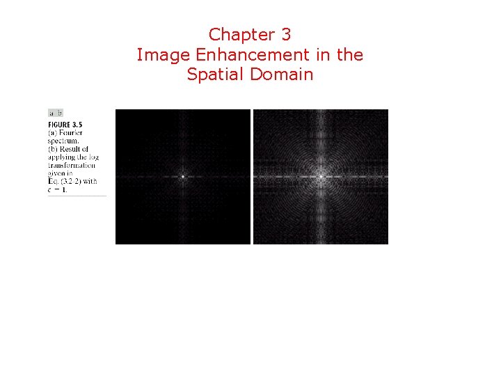
Log Transformation T(r) = c log(1+s) Inverse Log T(r) = exp(r/c)-1 For the next picture, c=1. Used to display Fourier spectra.

Chapter 3 Image Enhancement in the Spatial Domain

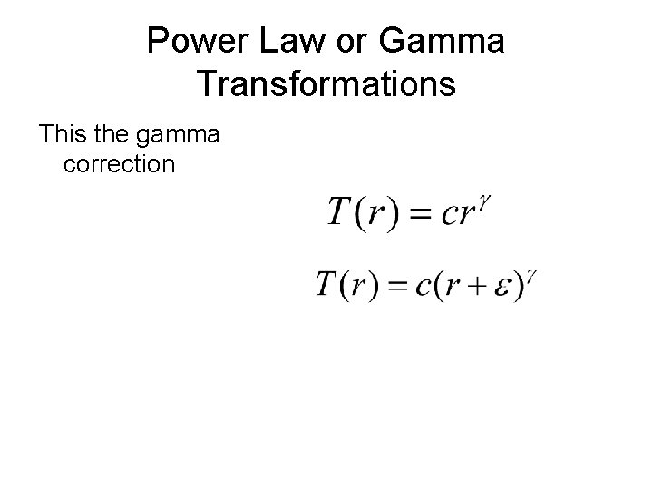
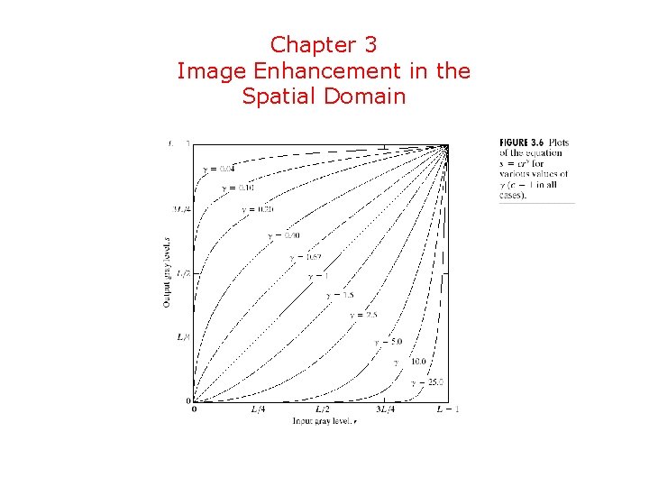
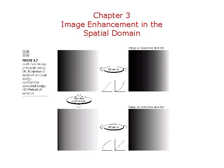
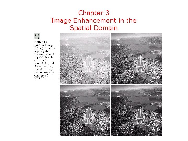
Power Law or Gamma Transformations This the gamma correction

Chapter 3 Image Enhancement in the Spatial Domain

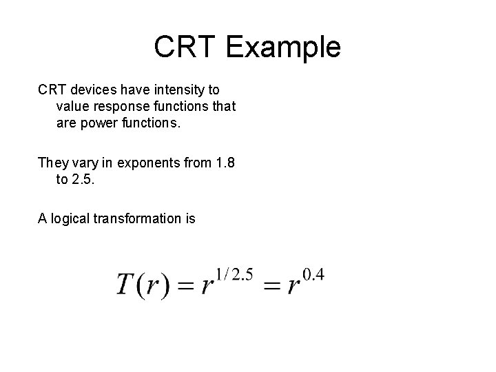
CRT Example CRT devices have intensity to value response functions that are power functions. They vary in exponents from 1. 8 to 2. 5. A logical transformation is

Chapter 3 Image Enhancement in the Spatial Domain

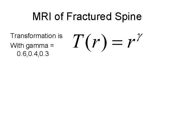
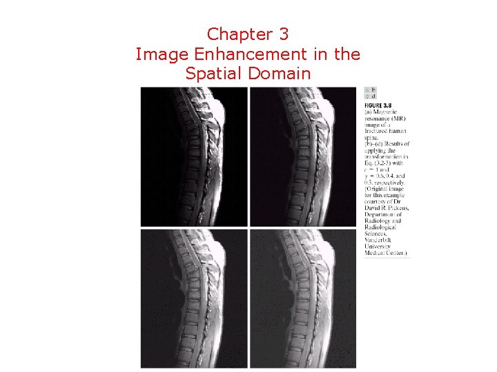
MRI of Fractured Spine Transformation is With gamma = 0. 6, 0. 4, 0. 3

Chapter 3 Image Enhancement in the Spatial Domain

Chapter 3 Image Enhancement in the Spatial Domain

Chapter 3 Image Enhancement in the Spatial Domain

Chapter 3 Image Enhancement in the Spatial Domain

Chapter 3 Image Enhancement in the Spatial Domain

Chapter 3 Image Enhancement in the Spatial Domain

Chapter 3 Image Enhancement in the Spatial Domain