Lecture Slides for INTRODUCTION TO Machine Learning ETHEM

Lecture Slides for INTRODUCTION TO Machine Learning ETHEM ALPAYDIN © The MIT Press, 2004 alpaydin@boun. edu. tr http: //www. cmpe. boun. edu. tr/~ethem/i 2 ml Lecture Notes for E Alpaydın 2004 Introduction to Machine Learning © The MIT Press (V 1. 1)

CHAPTER 9: Decision Trees Lecture Notes for E Alpaydın 2004 Introduction to Machine Learning © The MIT Press (V 1. 1)

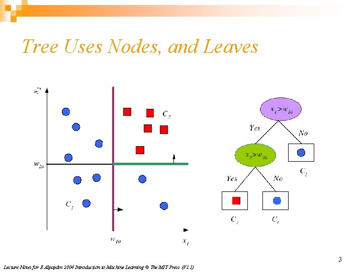
Tree Uses Nodes, and Leaves 3 Lecture Notes for E Alpaydın 2004 Introduction to Machine Learning © The MIT Press (V 1. 1)

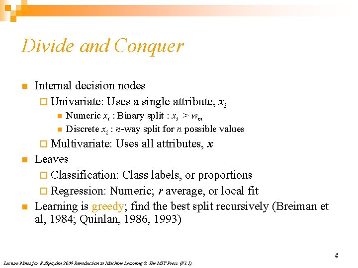
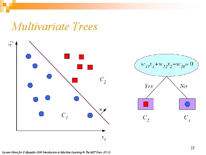
Divide and Conquer n Internal decision nodes ¨ Univariate: Uses a single attribute, xi n n Numeric xi : Binary split : xi > wm Discrete xi : n-way split for n possible values ¨ Multivariate: n n Uses all attributes, x Leaves ¨ Classification: Class labels, or proportions ¨ Regression: Numeric; r average, or local fit Learning is greedy; find the best split recursively (Breiman et al, 1984; Quinlan, 1986, 1993) 4 Lecture Notes for E Alpaydın 2004 Introduction to Machine Learning © The MIT Press (V 1. 1)

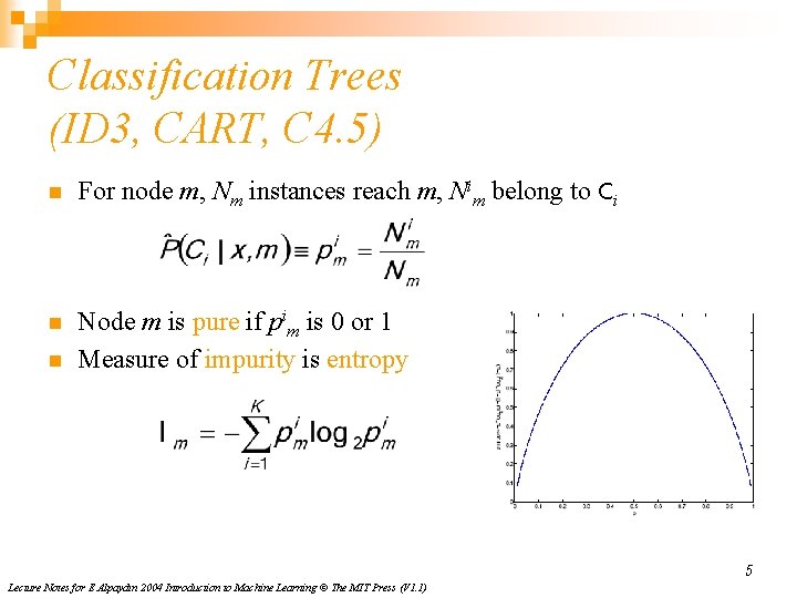
Classification Trees (ID 3, CART, C 4. 5) n For node m, Nm instances reach m, Nim belong to Ci n Node m is pure if pim is 0 or 1 Measure of impurity is entropy n 5 Lecture Notes for E Alpaydın 2004 Introduction to Machine Learning © The MIT Press (V 1. 1)

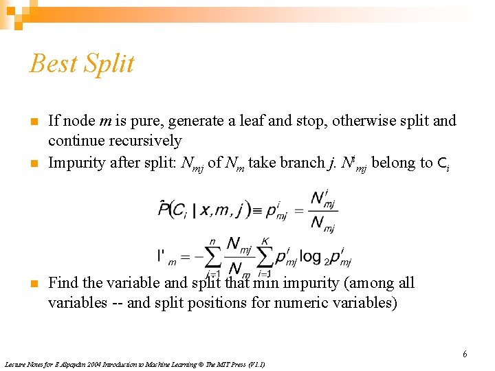
Best Split n n n If node m is pure, generate a leaf and stop, otherwise split and continue recursively Impurity after split: Nmj of Nm take branch j. Nimj belong to Ci Find the variable and split that min impurity (among all variables -- and split positions for numeric variables) 6 Lecture Notes for E Alpaydın 2004 Introduction to Machine Learning © The MIT Press (V 1. 1)

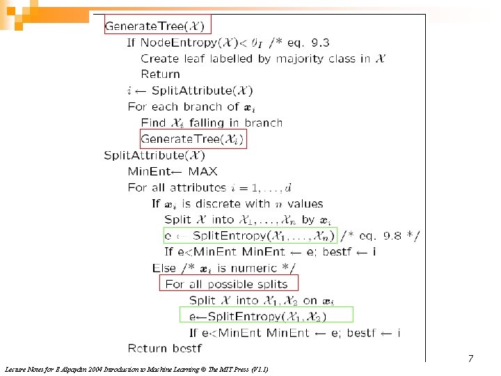
7 Lecture Notes for E Alpaydın 2004 Introduction to Machine Learning © The MIT Press (V 1. 1)

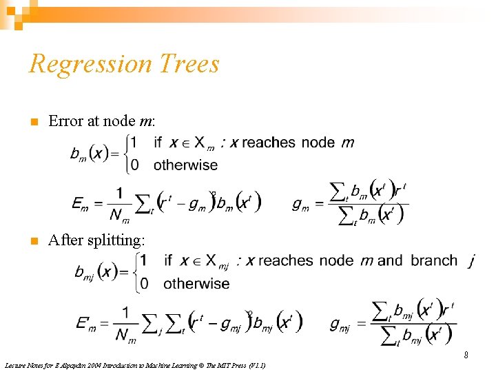
Regression Trees n Error at node m: n After splitting: 8 Lecture Notes for E Alpaydın 2004 Introduction to Machine Learning © The MIT Press (V 1. 1)

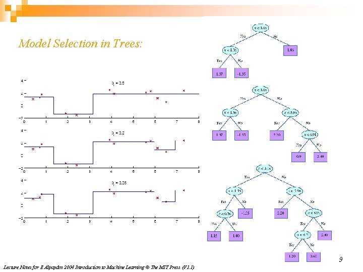
Model Selection in Trees: 9 Lecture Notes for E Alpaydın 2004 Introduction to Machine Learning © The MIT Press (V 1. 1)

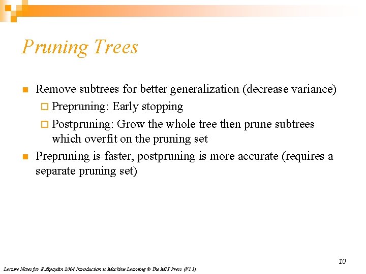
Pruning Trees n n Remove subtrees for better generalization (decrease variance) ¨ Prepruning: Early stopping ¨ Postpruning: Grow the whole tree then prune subtrees which overfit on the pruning set Prepruning is faster, postpruning is more accurate (requires a separate pruning set) 10 Lecture Notes for E Alpaydın 2004 Introduction to Machine Learning © The MIT Press (V 1. 1)

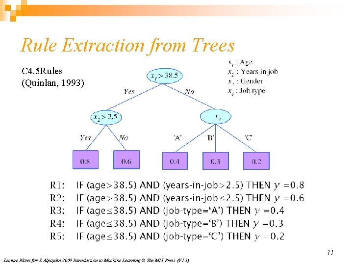
Rule Extraction from Trees C 4. 5 Rules (Quinlan, 1993) 11 Lecture Notes for E Alpaydın 2004 Introduction to Machine Learning © The MIT Press (V 1. 1)

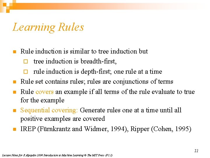
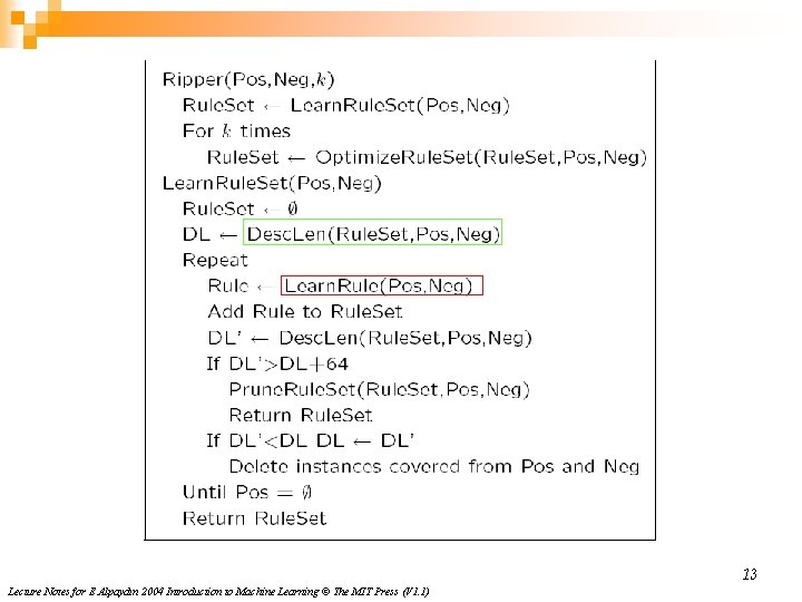
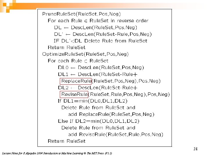
Learning Rules n n n Rule induction is similar to tree induction but ¨ tree induction is breadth-first, ¨ rule induction is depth-first; one rule at a time Rule set contains rules; rules are conjunctions of terms Rule covers an example if all terms of the rule evaluate to true for the example Sequential covering: Generate rules one at a time until all positive examples are covered IREP (Fürnkrantz and Widmer, 1994), Ripper (Cohen, 1995) 12 Lecture Notes for E Alpaydın 2004 Introduction to Machine Learning © The MIT Press (V 1. 1)

13 Lecture Notes for E Alpaydın 2004 Introduction to Machine Learning © The MIT Press (V 1. 1)

14 Lecture Notes for E Alpaydın 2004 Introduction to Machine Learning © The MIT Press (V 1. 1)

Multivariate Trees 15 Lecture Notes for E Alpaydın 2004 Introduction to Machine Learning © The MIT Press (V 1. 1)

Outline n n Decision tree representation ID 3 learning algorithm Entropy, information gain Overfitting 16 Lecture Notes for E Alpaydın 2004 Introduction to Machine Learning © The MIT Press (V 1. 1)

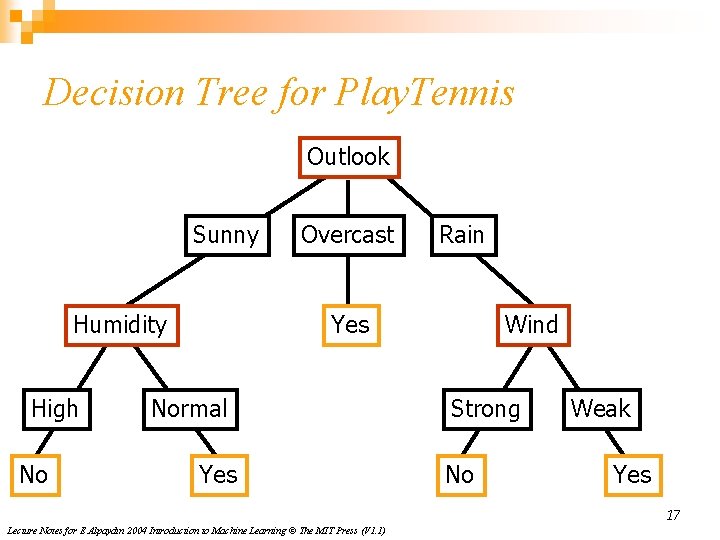
Decision Tree for Play. Tennis Outlook Sunny Humidity High No Overcast Rain Yes Normal Yes Wind Strong No Weak Yes 17 Lecture Notes for E Alpaydın 2004 Introduction to Machine Learning © The MIT Press (V 1. 1)

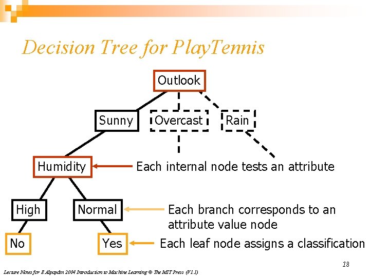
Decision Tree for Play. Tennis Outlook Sunny Humidity High No Overcast Rain Each internal node tests an attribute Normal Yes Each branch corresponds to an attribute value node Each leaf node assigns a classification 18 Lecture Notes for E Alpaydın 2004 Introduction to Machine Learning © The MIT Press (V 1. 1)

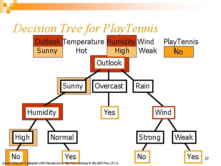
Decision Tree for Play. Tennis Outlook Temperature Humidity Wind Play. Tennis Sunny Hot High Weak ? No Outlook Sunny Humidity High No Overcast Rain Yes Normal Yes Lecture Notes for E Alpaydın 2004 Introduction to Machine Learning © The MIT Press (V 1. 1) Wind Strong No Weak Yes 19

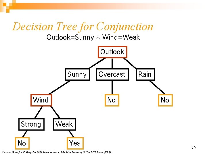
Decision Tree for Conjunction Outlook=Sunny Wind=Weak Outlook Sunny Wind Strong No Overcast No Rain No Weak Yes Lecture Notes for E Alpaydın 2004 Introduction to Machine Learning © The MIT Press (V 1. 1) 20

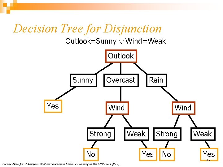
Decision Tree for Disjunction Outlook=Sunny Wind=Weak Outlook Sunny Yes Overcast Rain Wind Strong No Lecture Notes for E Alpaydın 2004 Introduction to Machine Learning © The MIT Press (V 1. 1) Wind Weak Yes Strong No Weak Yes 21

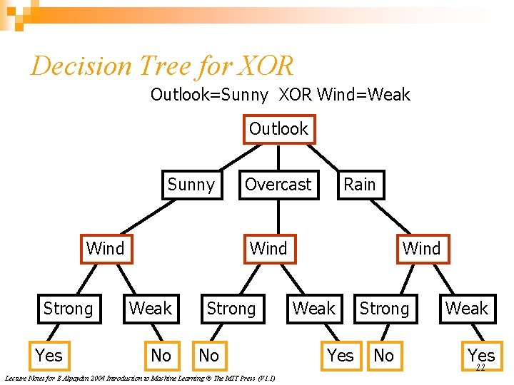
Decision Tree for XOR Outlook=Sunny XOR Wind=Weak Outlook Sunny Wind Strong Yes Overcast Rain Wind Weak No Strong No Lecture Notes for E Alpaydın 2004 Introduction to Machine Learning © The MIT Press (V 1. 1) Wind Weak Yes Strong No Weak Yes 22

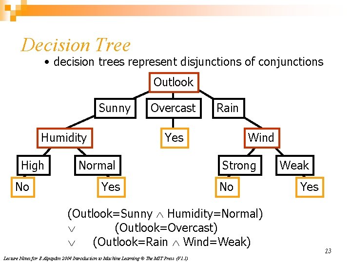
Decision Tree • decision trees represent disjunctions of conjunctions Outlook Sunny Humidity High No Overcast Rain Yes Normal Yes Wind Strong No (Outlook=Sunny Humidity=Normal) (Outlook=Overcast) (Outlook=Rain Wind=Weak) Lecture Notes for E Alpaydın 2004 Introduction to Machine Learning © The MIT Press (V 1. 1) Weak Yes 23

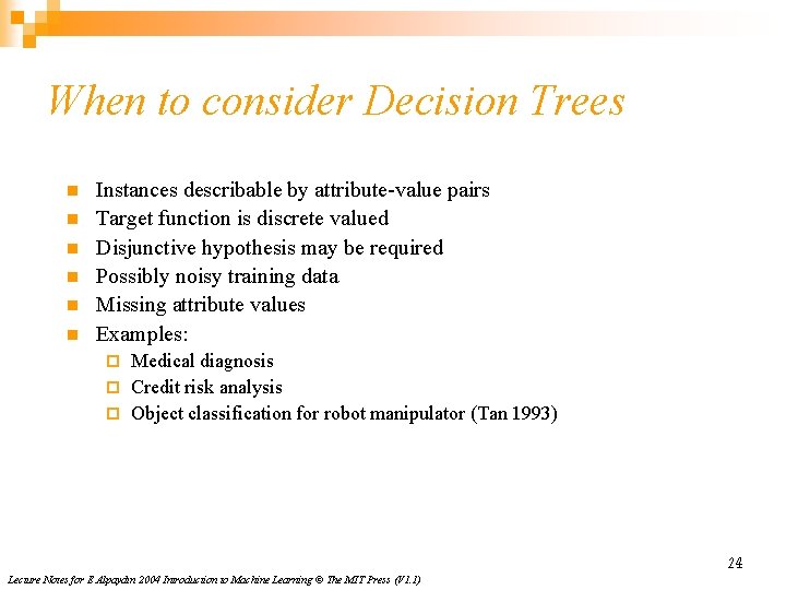
When to consider Decision Trees n n n Instances describable by attribute-value pairs Target function is discrete valued Disjunctive hypothesis may be required Possibly noisy training data Missing attribute values Examples: Medical diagnosis ¨ Credit risk analysis ¨ Object classification for robot manipulator (Tan 1993) ¨ 24 Lecture Notes for E Alpaydın 2004 Introduction to Machine Learning © The MIT Press (V 1. 1)

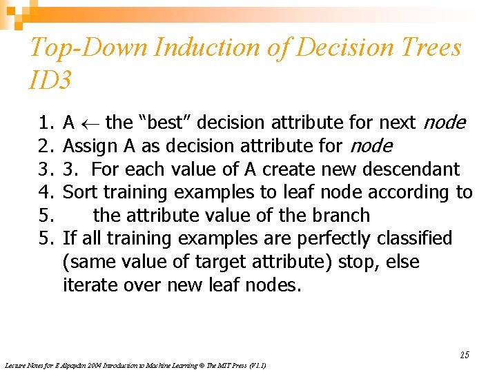
Top-Down Induction of Decision Trees ID 3 1. 2. 3. 4. 5. 5. A the “best” decision attribute for next node Assign A as decision attribute for node 3. For each value of A create new descendant Sort training examples to leaf node according to the attribute value of the branch If all training examples are perfectly classified (same value of target attribute) stop, else iterate over new leaf nodes. 25 Lecture Notes for E Alpaydın 2004 Introduction to Machine Learning © The MIT Press (V 1. 1)

Which Attribute is ”best”? [29+, 35 -] A 1=? True [21+, 5 -] A 2=? [29+, 35 -] False [8+, 30 -] True [18+, 33 -] False [11+, 2 -] 26 Lecture Notes for E Alpaydın 2004 Introduction to Machine Learning © The MIT Press (V 1. 1)

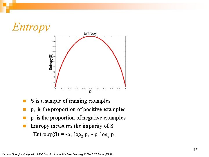
Entropy n n S is a sample of training examples p+ is the proportion of positive examples p- is the proportion of negative examples Entropy measures the impurity of S Entropy(S) = -p+ log 2 p+ - p- log 2 p 27 Lecture Notes for E Alpaydın 2004 Introduction to Machine Learning © The MIT Press (V 1. 1)

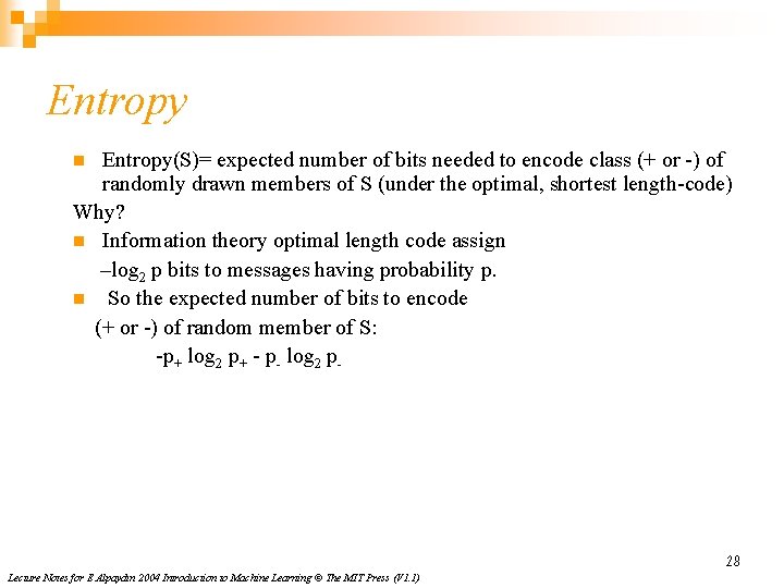
Entropy(S)= expected number of bits needed to encode class (+ or -) of randomly drawn members of S (under the optimal, shortest length-code) Why? n Information theory optimal length code assign –log 2 p bits to messages having probability p. n So the expected number of bits to encode (+ or -) of random member of S: -p+ log 2 p+ - p- log 2 pn 28 Lecture Notes for E Alpaydın 2004 Introduction to Machine Learning © The MIT Press (V 1. 1)

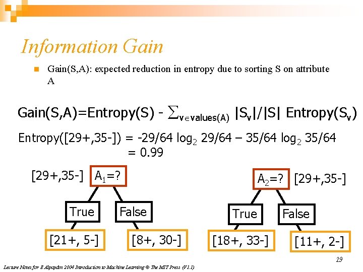
Information Gain(S, A): expected reduction in entropy due to sorting S on attribute A Gain(S, A)=Entropy(S) - v values(A) |Sv|/|S| Entropy(Sv) Entropy([29+, 35 -]) = -29/64 log 2 29/64 – 35/64 log 2 35/64 = 0. 99 [29+, 35 -] A 1=? True [21+, 5 -] A 2=? [29+, 35 -] False [8+, 30 -] True [18+, 33 -] False [11+, 2 -] 29 Lecture Notes for E Alpaydın 2004 Introduction to Machine Learning © The MIT Press (V 1. 1)

Information Gain Entropy([21+, 5 -]) = 0. 71 Entropy([8+, 30 -]) = 0. 74 Gain(S, A 1)=Entropy(S) -26/64*Entropy([21+, 5 -]) -38/64*Entropy([8+, 30 -]) =0. 27 Entropy([18+, 33 -]) = 0. 94 Entropy([8+, 30 -]) = 0. 62 Gain(S, A 2)=Entropy(S) -51/64*Entropy([18+, 33 -]) -13/64*Entropy([11+, 2 -]) =0. 12 [29+, 35 -] A 1=? True [21+, 5 -] A 2=? [29+, 35 -] False [8+, 30 -] Lecture Notes for E Alpaydın 2004 Introduction to Machine Learning © The MIT Press (V 1. 1) True [18+, 33 -] False [11+, 2 -] 30

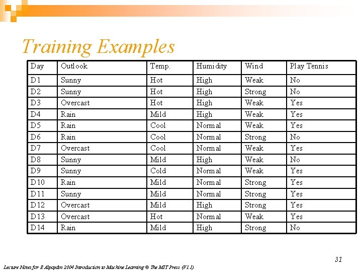
Training Examples Day Outlook Temp. Humidity Wind Play Tennis D 1 D 2 D 3 D 4 D 5 D 6 D 7 D 8 D 9 D 10 D 11 D 12 D 13 D 14 Sunny Overcast Rain Overcast Sunny Rain Sunny Overcast Rain Hot Hot Mild Cool Mild Cold Mild Hot Mild High Normal Normal High Weak Strong Weak Weak Strong Weak Strong No No Yes Yes Yes No 31 Lecture Notes for E Alpaydın 2004 Introduction to Machine Learning © The MIT Press (V 1. 1)

Selecting the Next Attribute S=[9+, 5 -] E=0. 940 Humidity Wind High [3+, 4 -] E=0. 985 Normal Weak Strong [6+, 1 -] [6+, 2 -] E=0. 592 E=0. 811 E=1. 0 Gain(S, Wind) =0. 940 -(8/14)*0. 811 – (6/14)*1. 0 =0. 048 Gain(S, Humidity) =0. 940 -(7/14)*0. 985 – (7/14)*0. 592 =0. 151 Lecture Notes for E Alpaydın 2004 Introduction to Machine Learning © The MIT Press (V 1. 1) [3+, 3 -] 32

Selecting the Next Attribute S=[9+, 5 -] E=0. 940 Outlook Sunny Over cast Rain [2+, 3 -] [4+, 0] [3+, 2 -] E=0. 971 E=0. 0 E=0. 971 Gain(S, Outlook) =0. 940 -(5/14)*0. 971 -(4/14)*0. 0 – (5/14)*0. 0971 =0. 247 Lecture Notes for E Alpaydın 2004 Introduction to Machine Learning © The MIT Press (V 1. 1) 33

ID 3 Algorithm [D 1, D 2, …, D 14] [9+, 5 -] Outlook Sunny Overcast Rain Ssunny=[D 1, D 2, D 8, D 9, D 11] [D 3, D 7, D 12, D 13] [D 4, D 5, D 6, D 10, D 14] [2+, 3 -] [4+, 0 -] [3+, 2 -] ? Yes ? Gain(Ssunny , Humidity)=0. 970 -(3/5)0. 0 – 2/5(0. 0) = 0. 970 Gain(Ssunny , Temp. )=0. 970 -(2/5)0. 0 – 2/5(1. 0)-(1/5)0. 0 = 0. 570 Gain(Ssunny , Wind)=0. 970= -(2/5)1. 0 – 3/5(0. 918) = 0. 019 34 Lecture Notes for E Alpaydın 2004 Introduction to Machine Learning © The MIT Press (V 1. 1)

ID 3 Algorithm Outlook Sunny Humidity High No [D 1, D 2] Overcast Rain Yes [D 3, D 7, D 12, D 13] Normal Yes [D 8, D 9, D 11] Lecture Notes for E Alpaydın 2004 Introduction to Machine Learning © The MIT Press (V 1. 1) Wind Strong Weak No Yes [D 6, D 14] [D 4, D 5, D 10] 35

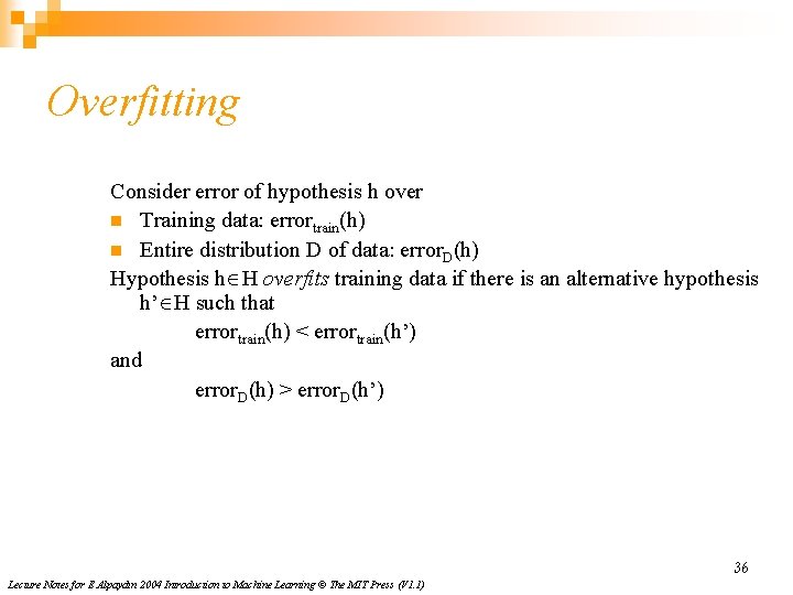
Overfitting Consider error of hypothesis h over n Training data: errortrain(h) n Entire distribution D of data: error. D(h) Hypothesis h H overfits training data if there is an alternative hypothesis h’ H such that errortrain(h) < errortrain(h’) and error. D(h) > error. D(h’) 36 Lecture Notes for E Alpaydın 2004 Introduction to Machine Learning © The MIT Press (V 1. 1)

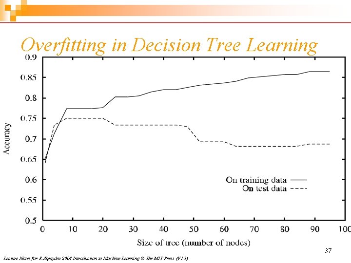
Overfitting in Decision Tree Learning 37 Lecture Notes for E Alpaydın 2004 Introduction to Machine Learning © The MIT Press (V 1. 1)

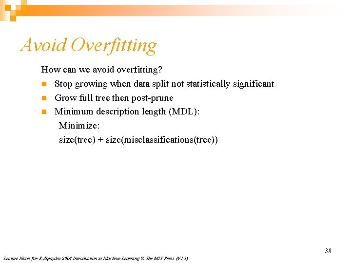
Avoid Overfitting How can we avoid overfitting? n Stop growing when data split not statistically significant n Grow full tree then post-prune n Minimum description length (MDL): Minimize: size(tree) + size(misclassifications(tree)) 38 Lecture Notes for E Alpaydın 2004 Introduction to Machine Learning © The MIT Press (V 1. 1)

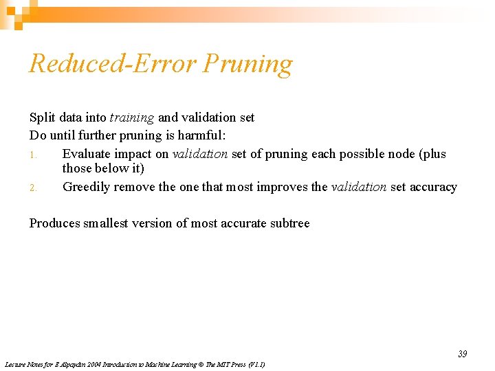
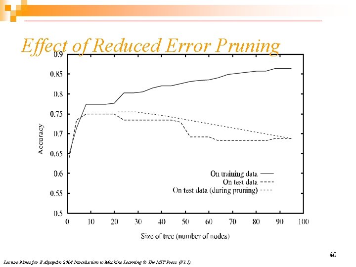
Reduced-Error Pruning Split data into training and validation set Do until further pruning is harmful: 1. Evaluate impact on validation set of pruning each possible node (plus those below it) 2. Greedily remove the one that most improves the validation set accuracy Produces smallest version of most accurate subtree 39 Lecture Notes for E Alpaydın 2004 Introduction to Machine Learning © The MIT Press (V 1. 1)

Effect of Reduced Error Pruning 40 Lecture Notes for E Alpaydın 2004 Introduction to Machine Learning © The MIT Press (V 1. 1)

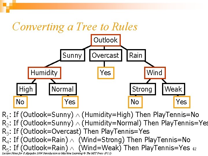
Rule-Post Pruning 1. 2. 3. Convert tree to equivalent set of rules Prune each rule independently of each other Sort final rules into a desired sequence to use Method used in C 4. 5 41 Lecture Notes for E Alpaydın 2004 Introduction to Machine Learning © The MIT Press (V 1. 1)

Converting a Tree to Rules Outlook Sunny Humidity High No R 1: R 2: R 3: R 4: R 5: If If If Overcast Rain Yes Normal Yes Wind Strong No Weak Yes (Outlook=Sunny) (Humidity=High) Then Play. Tennis=No (Outlook=Sunny) (Humidity=Normal) Then Play. Tennis=Yes (Outlook=Overcast) Then Play. Tennis=Yes (Outlook=Rain) (Wind=Strong) Then Play. Tennis=No (Outlook=Rain) (Wind=Weak) Then Play. Tennis=Yes 42 Lecture Notes for E Alpaydın 2004 Introduction to Machine Learning © The MIT Press (V 1. 1)

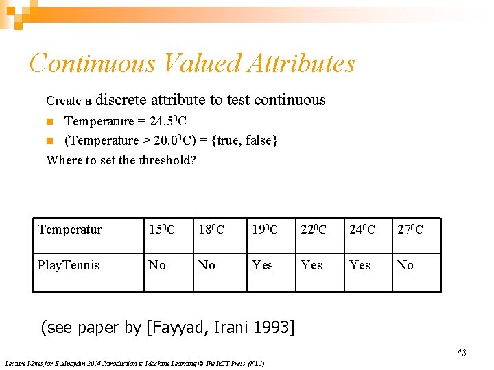
Continuous Valued Attributes Create a discrete attribute to test continuous n Temperature = 24. 50 C n (Temperature > 20. 00 C) = {true, false} Where to set the threshold? Temperatur 150 C 180 C 190 C 220 C 240 C 270 C Play. Tennis No No Yes Yes No (see paper by [Fayyad, Irani 1993] 43 Lecture Notes for E Alpaydın 2004 Introduction to Machine Learning © The MIT Press (V 1. 1)

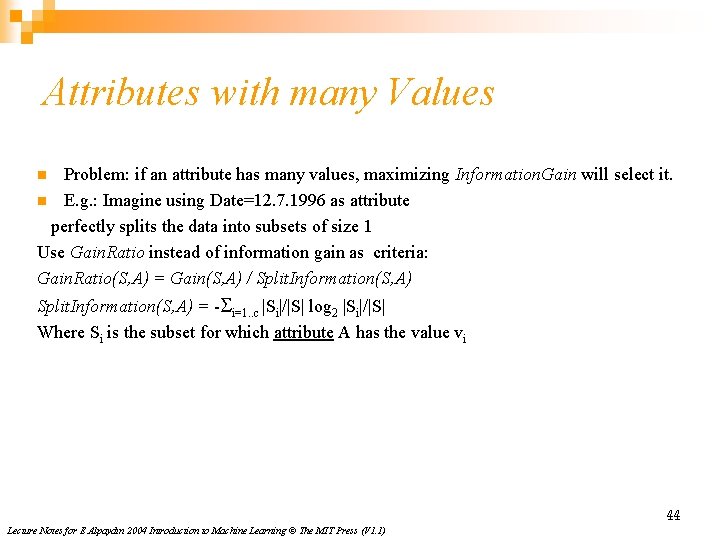
Attributes with many Values Problem: if an attribute has many values, maximizing Information. Gain will select it. n E. g. : Imagine using Date=12. 7. 1996 as attribute perfectly splits the data into subsets of size 1 Use Gain. Ratio instead of information gain as criteria: Gain. Ratio(S, A) = Gain(S, A) / Split. Information(S, A) n Split. Information(S, A) = - i=1. . c |Si|/|S| log 2 |Si|/|S| Where Si is the subset for which attribute A has the value vi 44 Lecture Notes for E Alpaydın 2004 Introduction to Machine Learning © The MIT Press (V 1. 1)

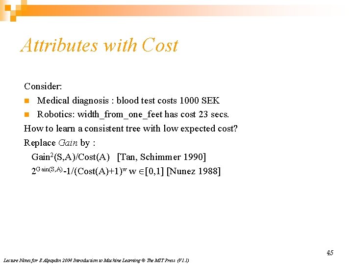
Attributes with Cost Consider: n Medical diagnosis : blood test costs 1000 SEK n Robotics: width_from_one_feet has cost 23 secs. How to learn a consistent tree with low expected cost? Replace Gain by : Gain 2(S, A)/Cost(A) [Tan, Schimmer 1990] 2 Gain(S, A)-1/(Cost(A)+1)w w [0, 1] [Nunez 1988] 45 Lecture Notes for E Alpaydın 2004 Introduction to Machine Learning © The MIT Press (V 1. 1)

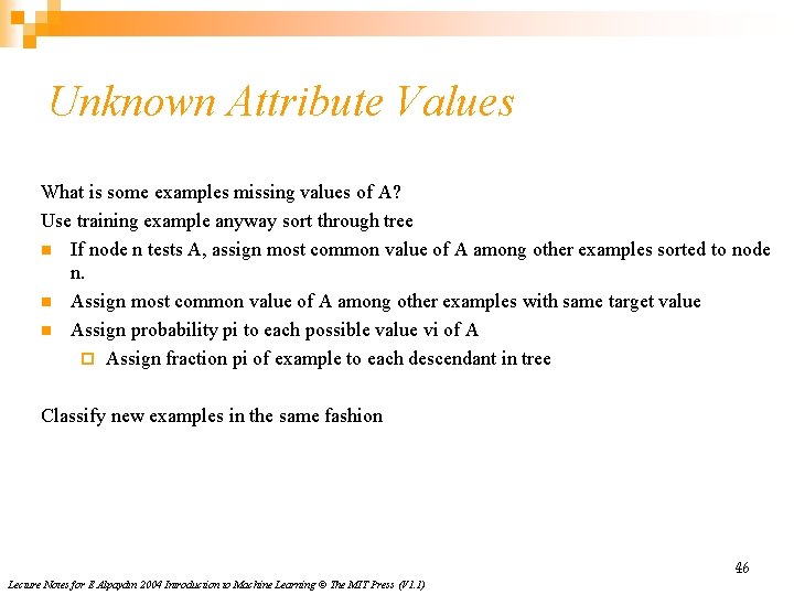
Unknown Attribute Values What is some examples missing values of A? Use training example anyway sort through tree n If node n tests A, assign most common value of A among other examples sorted to node n. n Assign most common value of A among other examples with same target value n Assign probability pi to each possible value vi of A ¨ Assign fraction pi of example to each descendant in tree Classify new examples in the same fashion 46 Lecture Notes for E Alpaydın 2004 Introduction to Machine Learning © The MIT Press (V 1. 1)

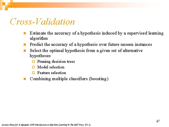
Cross-Validation n Estimate the accuracy of a hypothesis induced by a supervised learning algorithm Predict the accuracy of a hypothesis over future unseen instances Select the optimal hypothesis from a given set of alternative hypotheses Pruning decision trees ¨ Model selection ¨ Feature selection ¨ n Combining multiple classifiers (boosting) 47 Lecture Notes for E Alpaydın 2004 Introduction to Machine Learning © The MIT Press (V 1. 1)

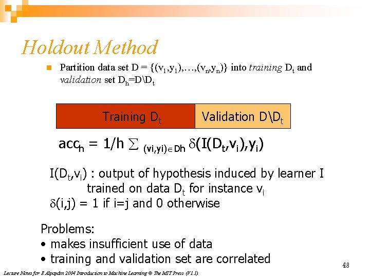
Holdout Method n Partition data set D = {(v 1, y 1), …, (vn, yn)} into training Dt and validation set Dh=DDt Training Dt acch = 1/h (vi, yi) Dh Validation DDt (I(Dt, vi), yi) I(Dt, vi) : output of hypothesis induced by learner I trained on data Dt for instance vi (i, j) = 1 if i=j and 0 otherwise Problems: • makes insufficient use of data • training and validation set are correlated Lecture Notes for E Alpaydın 2004 Introduction to Machine Learning © The MIT Press (V 1. 1) 48

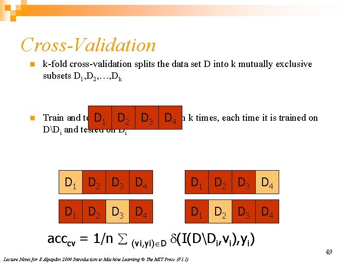
Cross-Validation n k-fold cross-validation splits the data set D into k mutually exclusive subsets D 1, D 2, …, Dk n Train and test. Dthe learning algorithm k times, each time it is trained on 1 D 2 D 3 D 4 DDi and tested on Di D 1 D 2 D 3 D 4 acccv = 1/n (vi, yi) D (I(DDi, vi), yi) Lecture Notes for E Alpaydın 2004 Introduction to Machine Learning © The MIT Press (V 1. 1) 49

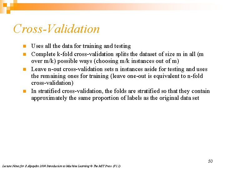
Cross-Validation n n Uses all the data for training and testing Complete k-fold cross-validation splits the dataset of size m in all (m over m/k) possible ways (choosing m/k instances out of m) Leave n-out cross-validation sets n instances aside for testing and uses the remaining ones for training (leave one-out is equivalent to n-fold cross-validation) In stratified cross-validation, the folds are stratified so that they contain approximately the same proportion of labels as the original data set 50 Lecture Notes for E Alpaydın 2004 Introduction to Machine Learning © The MIT Press (V 1. 1)

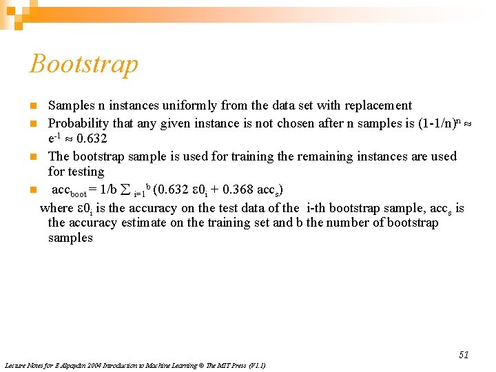
Bootstrap Samples n instances uniformly from the data set with replacement n Probability that any given instance is not chosen after n samples is (1 -1/n)n e-1 0. 632 n The bootstrap sample is used for training the remaining instances are used for testing n accboot = 1/b i=1 b (0. 632 0 i + 0. 368 accs) where 0 i is the accuracy on the test data of the i-th bootstrap sample, accs is the accuracy estimate on the training set and b the number of bootstrap samples n 51 Lecture Notes for E Alpaydın 2004 Introduction to Machine Learning © The MIT Press (V 1. 1)