Lecture Slides for INTRODUCTION TO Machine Learning ETHEM

Lecture Slides for INTRODUCTION TO Machine Learning ETHEM ALPAYDIN © The MIT Press, 2004 alpaydin@boun. edu. tr http: //www. cmpe. boun. edu. tr/~ethem/i 2 ml

CHAPTER 11: Multilayer Perceptrons

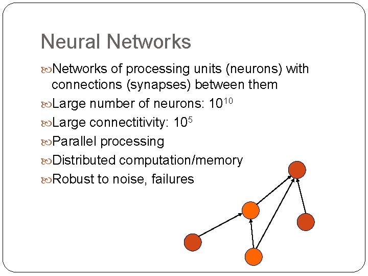
Neural Networks of processing units (neurons) with connections (synapses) between them Large number of neurons: 1010 Large connectitivity: 105 Parallel processing Distributed computation/memory Robust to noise, failures 3

Understanding the Brain Levels of analysis (Marr, 1982) 1. Computational theory 2. Representation and algorithm 3. Hardware implementation Reverse engineering: From hardware to theory Parallel processing: SIMD vs MIMD Neural net: SIMD with modifiable local memory Learning: Update by training/experience 4

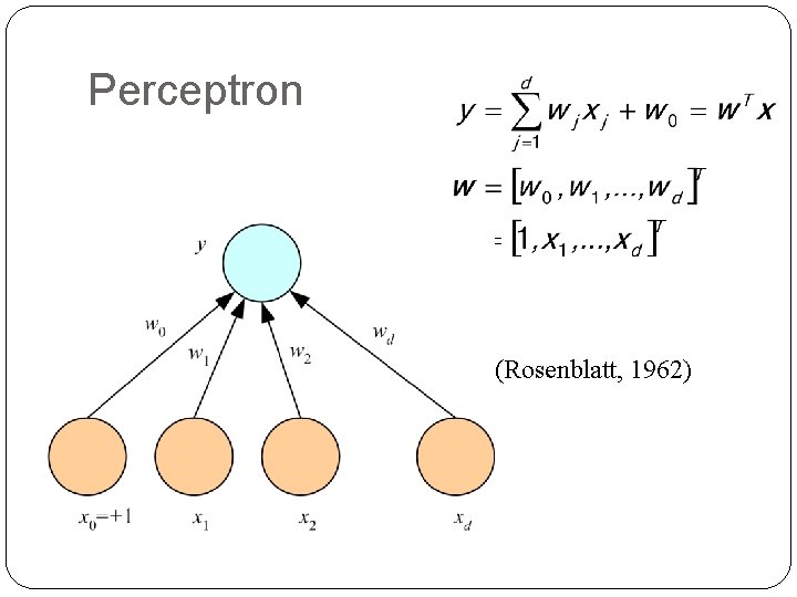
Perceptron (Rosenblatt, 1962) 5

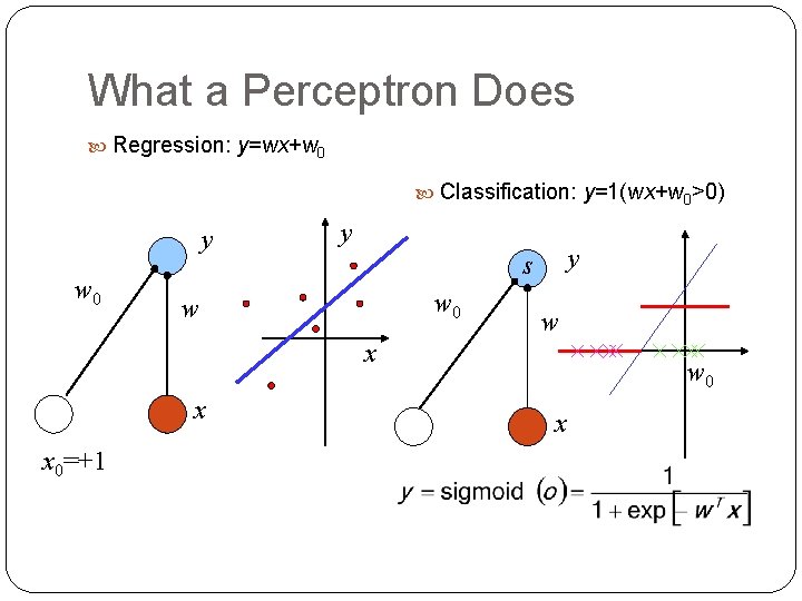
What a Perceptron Does Regression: y=wx+w 0 Classification: y=1(wx+w 0>0) y w 0 y y s w 0 w w x x x 0=+1 6 w 0 x

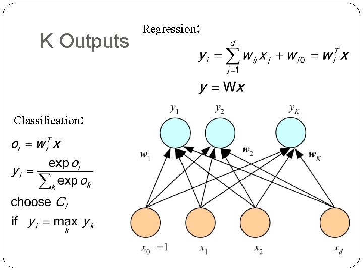
K Outputs Classification: 7 Regression:

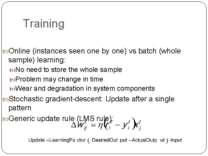
Training Online (instances seen one by one) vs batch (whole sample) learning: No need to store the whole sample Problem may change in time Wear and degradation in system components Stochastic gradient-descent: Update after a single pattern Generic update rule (LMS rule): 8

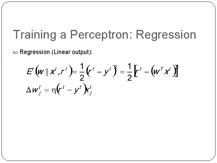
Training a Perceptron: Regression (Linear output): 9

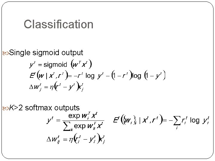
Classification Single sigmoid output K>2 softmax outputs 10

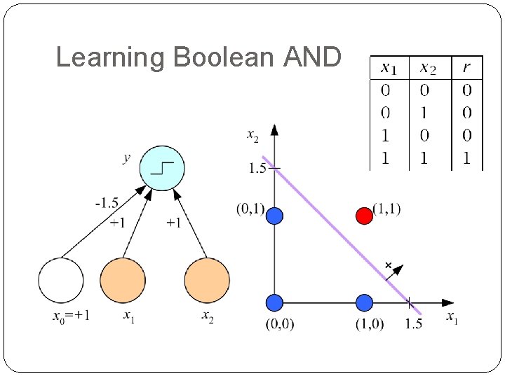
Learning Boolean AND 11

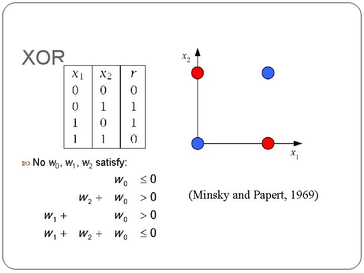
XOR No w 0, w 1, w 2 satisfy: (Minsky and Papert, 1969) 12

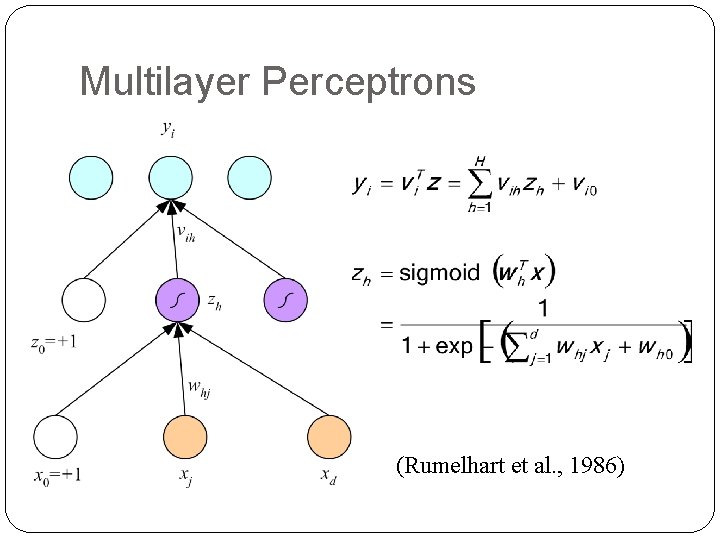
Multilayer Perceptrons (Rumelhart et al. , 1986) 13

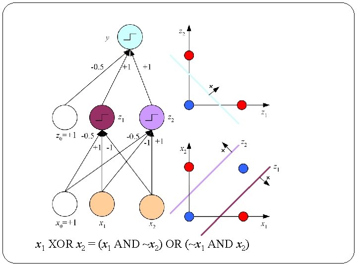
14 x 1 XOR x 2 = (x 1 AND ~x 2) OR (~x 1 AND x 2)

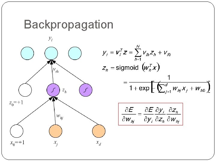
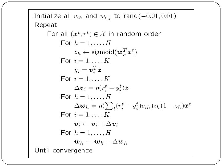
Backpropagation 15

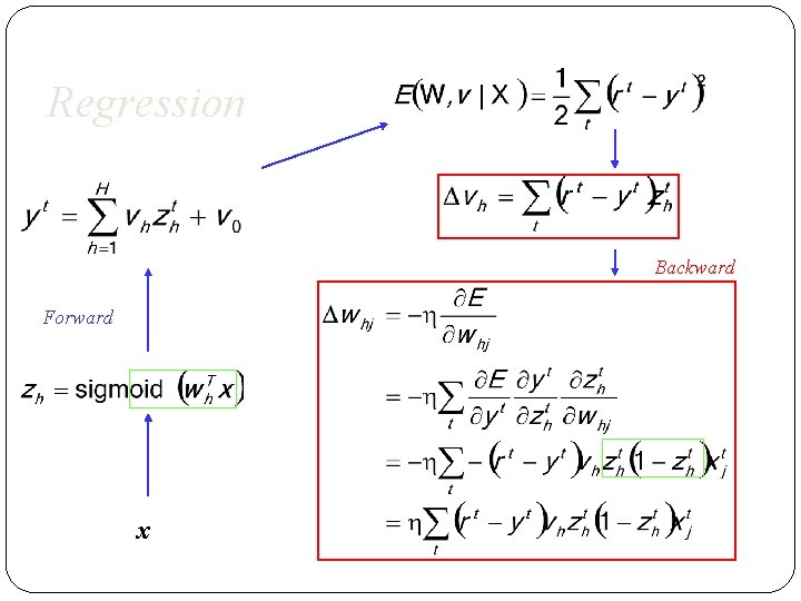
Regression Backward Forward x 16

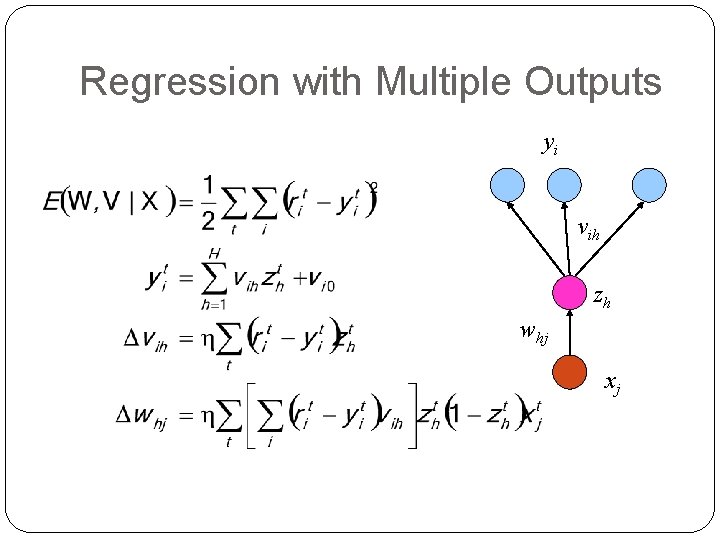
Regression with Multiple Outputs yi vih zh whj xj 17

18

19

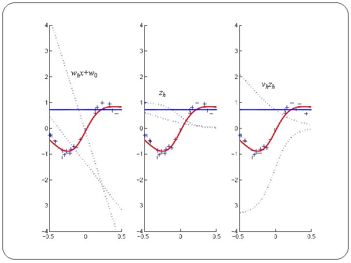
whx+w 0 zh 20 v h zh

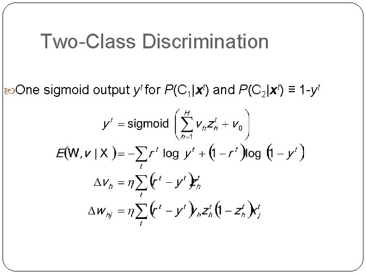
Two-Class Discrimination One sigmoid output yt for P(C 1|xt) and P(C 2|xt) ≡ 1 -yt 21

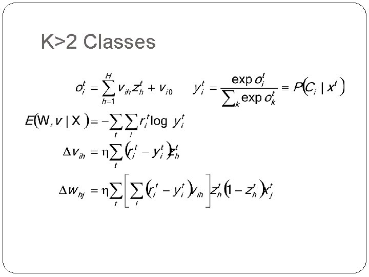
K>2 Classes 22

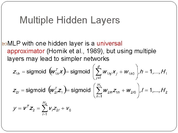
Multiple Hidden Layers MLP with one hidden layer is a universal approximator (Hornik et al. , 1989), but using multiple layers may lead to simpler networks 23

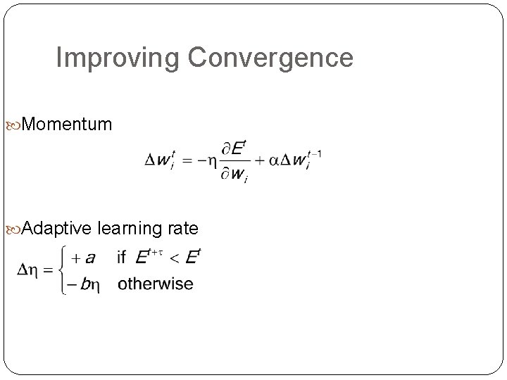
Improving Convergence Momentum Adaptive learning rate 24

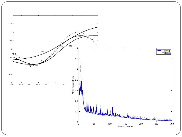
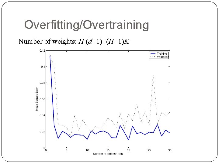
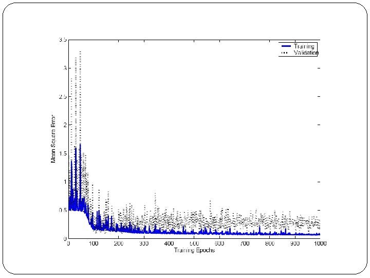
Overfitting/Overtraining Number of weights: H (d+1)+(H+1)K 25

26

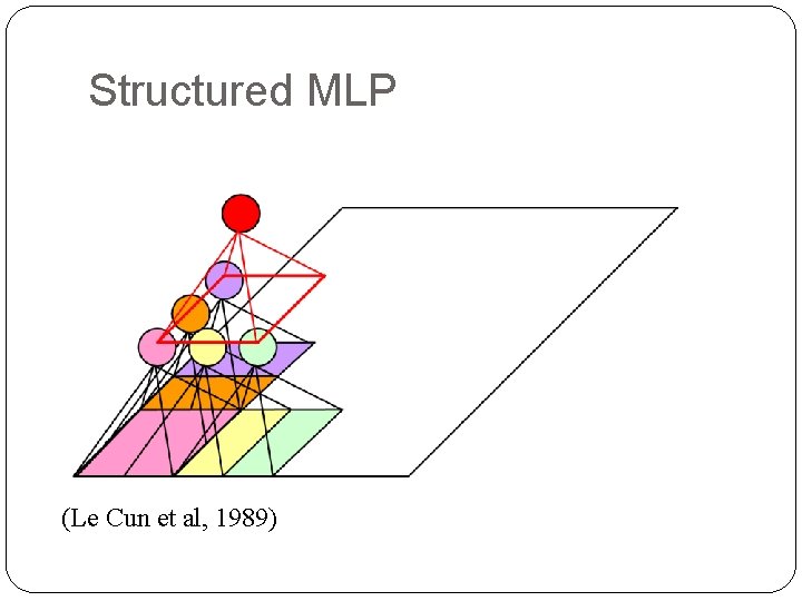
Structured MLP (Le Cun et al, 1989) 27

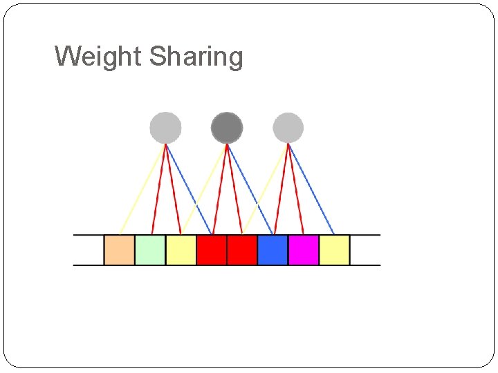
Weight Sharing 28

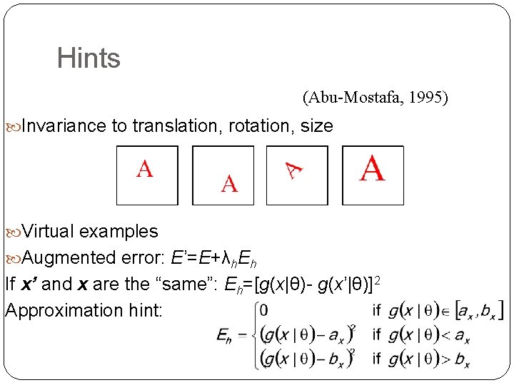
Hints (Abu-Mostafa, 1995) Invariance to translation, rotation, size Virtual examples Augmented error: E’=E+λh. Eh If x’ and x are the “same”: Eh=[g(x|θ)- g(x’|θ)]2 Approximation hint: 29

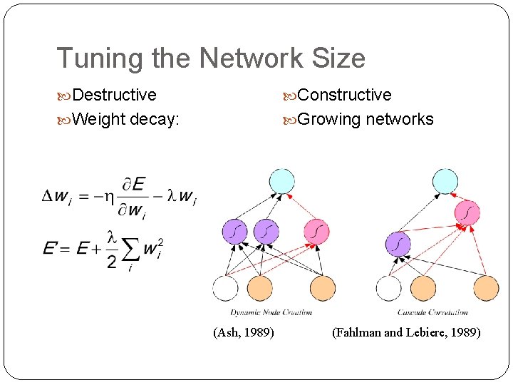
Tuning the Network Size Destructive Constructive Weight decay: Growing networks (Ash, 1989) 30 (Fahlman and Lebiere, 1989)

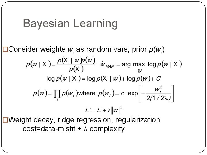
Bayesian Learning �Consider weights wi as random vars, prior p(wi) �Weight decay, ridge regression, regularization cost=data-misfit + λ complexity 31

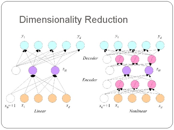
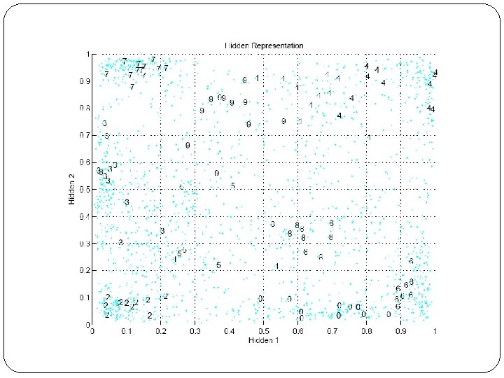
Dimensionality Reduction 32

33

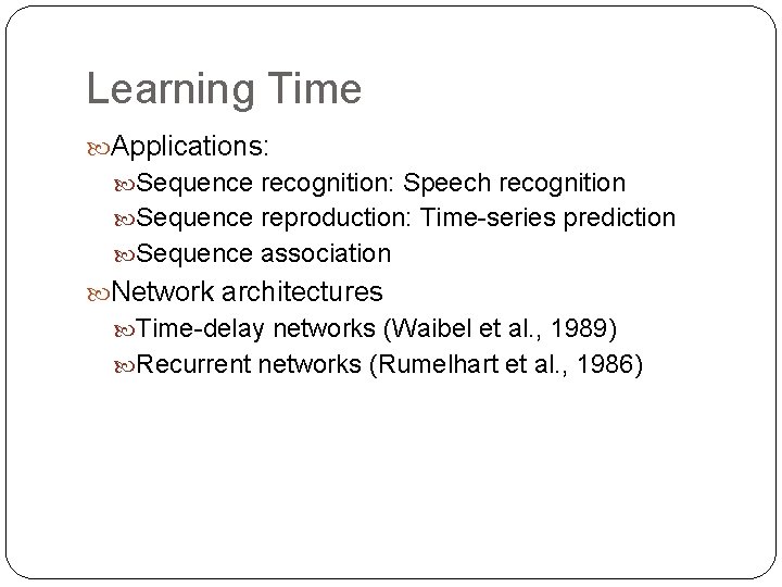
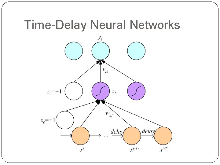
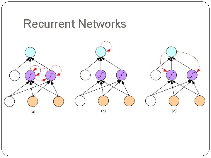
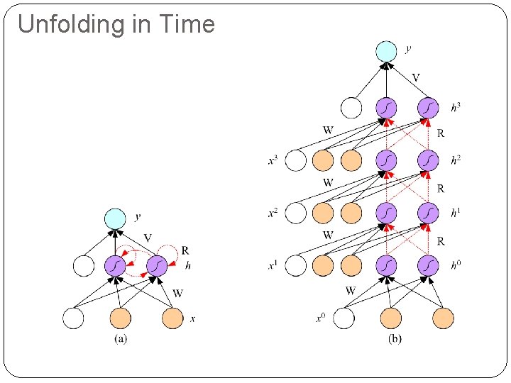
Learning Time Applications: Sequence recognition: Speech recognition Sequence reproduction: Time-series prediction Sequence association Network architectures Time-delay networks (Waibel et al. , 1989) Recurrent networks (Rumelhart et al. , 1986) 34

Time-Delay Neural Networks 35

Recurrent Networks 36

Unfolding in Time 37