Lecture Slides for INTRODUCTION TO Machine Learning ETHEM

Lecture Slides for INTRODUCTION TO Machine Learning ETHEM ALPAYDIN © The MIT Press, 2004 alpaydin@boun. edu. tr http: //www. cmpe. boun. edu. tr/~ethem/i 2 ml

CHAPTER 10: Linear Discrimination CHAPTER 13: Support Vector Machines

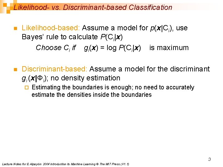
Likelihood- vs. Discriminant-based Classification n Likelihood-based: Assume a model for p(x|Ci), use Bayes’ rule to calculate P(Ci|x) Choose Ci if gi(x) = log P(Ci|x) is maximum n Discriminant-based: Assume a model for the discriminant gi (x|Φi); no density estimation ¨ Estimating the boundaries is enough; no need to accurately estimate the densities inside the boundaries 3 Lecture Notes for E Alpaydın 2004 Introduction to Machine Learning © The MIT Press (V 1. 1)

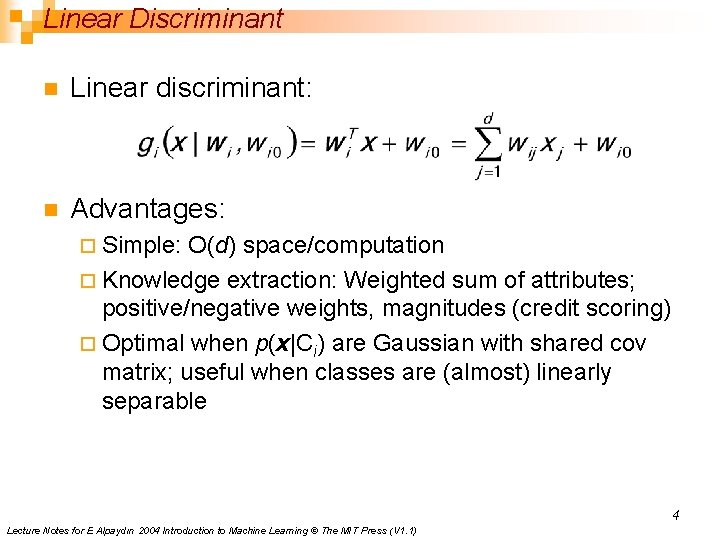
Linear Discriminant n Linear discriminant: n Advantages: ¨ Simple: O(d) space/computation ¨ Knowledge extraction: Weighted sum of attributes; positive/negative weights, magnitudes (credit scoring) ¨ Optimal when p(x|Ci) are Gaussian with shared cov matrix; useful when classes are (almost) linearly separable 4 Lecture Notes for E Alpaydın 2004 Introduction to Machine Learning © The MIT Press (V 1. 1)

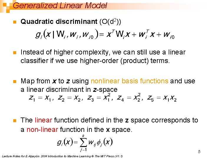
Generalized Linear Model n Quadratic discriminant (O(d 2)) n Instead of higher complexity, we can still use a linear classifier if we use higher-order (product) terms. n Map from x to z using nonlinear basis functions and use a linear discriminant in z-space n The linear function defined in the z space corresponds to a non-linear function in the x space. 5 Lecture Notes for E Alpaydın 2004 Introduction to Machine Learning © The MIT Press (V 1. 1)

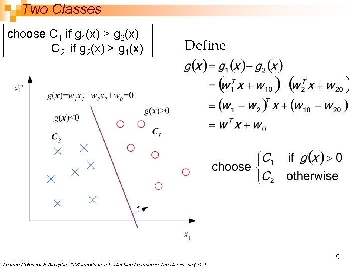
Two Classes choose C 1 if g 1(x) > g 2(x) C 2 if g 2(x) > g 1(x) Define: 6 Lecture Notes for E Alpaydın 2004 Introduction to Machine Learning © The MIT Press (V 1. 1)

A Bit of Geometry

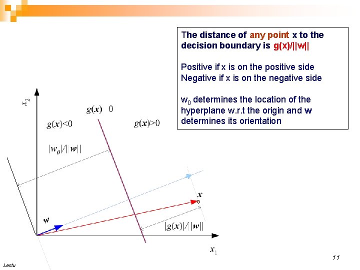
The distance of any point x to the decision boundary is g(x)/||w|| Positive if x is on the positive side Negative if x is on the negative side w 0 determines the location of the hyperplane w. r. t the origin and w determines its orientation 11 Lecture Notes for E Alpaydın 2004 Introduction to Machine Learning © The MIT Press (V 1. 1)

How to Deal with Multi-class Problems Lecture Notes for E Alpaydın 2004 Introduction to Machine Learning © The MIT Press (V 1. 1)

n When K > 2 ¨ Combine K two-class problems, each one separating one class from all other classes 13 Lecture Notes for E Alpaydın 2004 Introduction to Machine Learning © The MIT Press (V 1. 1)

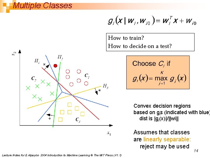
Multiple Classes How to train? How to decide on a test? Convex decision regions based on gis (indicated with blue) dist is |gi(x)|/||wi|| Assumes that classes are linearly separable: reject may be used Lecture Notes for E Alpaydın 2004 Introduction to Machine Learning © The MIT Press (V 1. 1) 14

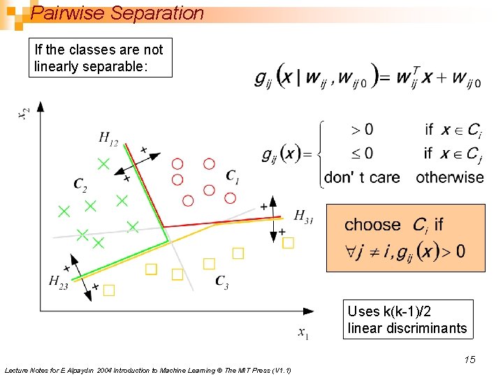
Pairwise Separation If the classes are not linearly separable: Uses k(k-1)/2 linear discriminants 15 Lecture Notes for E Alpaydın 2004 Introduction to Machine Learning © The MIT Press (V 1. 1)

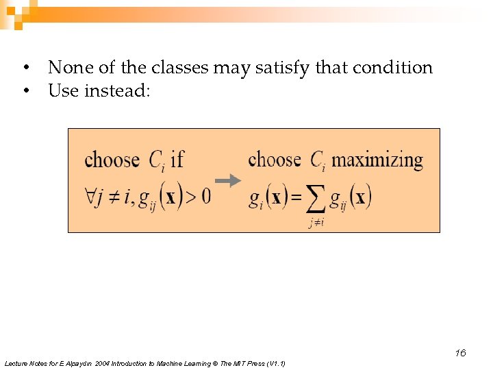
• None of the classes may satisfy that condition • Use instead: 16 Lecture Notes for E Alpaydın 2004 Introduction to Machine Learning © The MIT Press (V 1. 1)

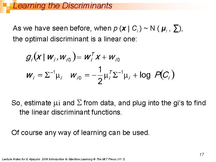
Learning the Discriminants As we have seen before, when p (x | Ci ) ~ N ( μi , ∑), the optimal discriminant is a linear one: So, estimate mi and S from data, and plug into the gi’s to find the linear discriminant functions. Of course any way of learning can be used. 17 Lecture Notes for E Alpaydın 2004 Introduction to Machine Learning © The MIT Press (V 1. 1)

Support Vector Machines

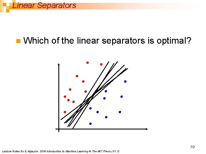
Linear Separators n Which of the linear separators is optimal? 19 Lecture Notes for E Alpaydın 2004 Introduction to Machine Learning © The MIT Press (V 1. 1)

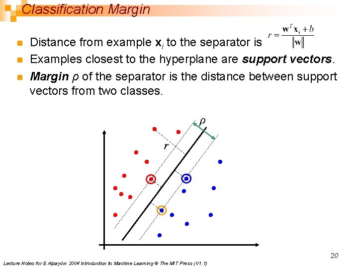
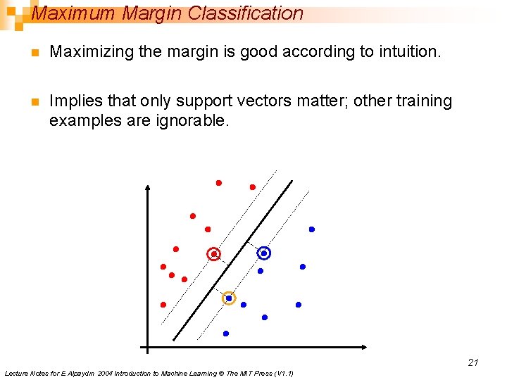
Classification Margin n Distance from example xi to the separator is Examples closest to the hyperplane are support vectors. Margin ρ of the separator is the distance between support vectors from two classes. ρ r 20 Lecture Notes for E Alpaydın 2004 Introduction to Machine Learning © The MIT Press (V 1. 1)

Maximum Margin Classification n Maximizing the margin is good according to intuition. n Implies that only support vectors matter; other training examples are ignorable. 21 Lecture Notes for E Alpaydın 2004 Introduction to Machine Learning © The MIT Press (V 1. 1)

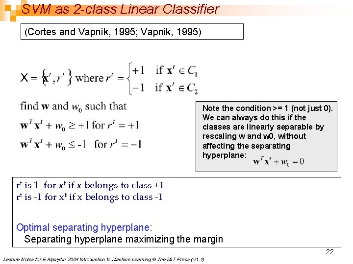
SVM as 2 -class Linear Classifier (Cortes and Vapnik, 1995; Vapnik, 1995) Note the condition >= 1 (not just 0). We can always do this if the classes are linearly separable by rescaling w and w 0, without affecting the separating hyperplane: rt is 1 for xt if x belongs to class +1 rt is -1 for xt if x belongs to class -1 Optimal separating hyperplane: Separating hyperplane maximizing the margin 22 Lecture Notes for E Alpaydın 2004 Introduction to Machine Learning © The MIT Press (V 1. 1)

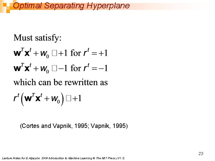
Optimal Separating Hyperplane (Cortes and Vapnik, 1995; Vapnik, 1995) 23 Lecture Notes for E Alpaydın 2004 Introduction to Machine Learning © The MIT Press (V 1. 1)

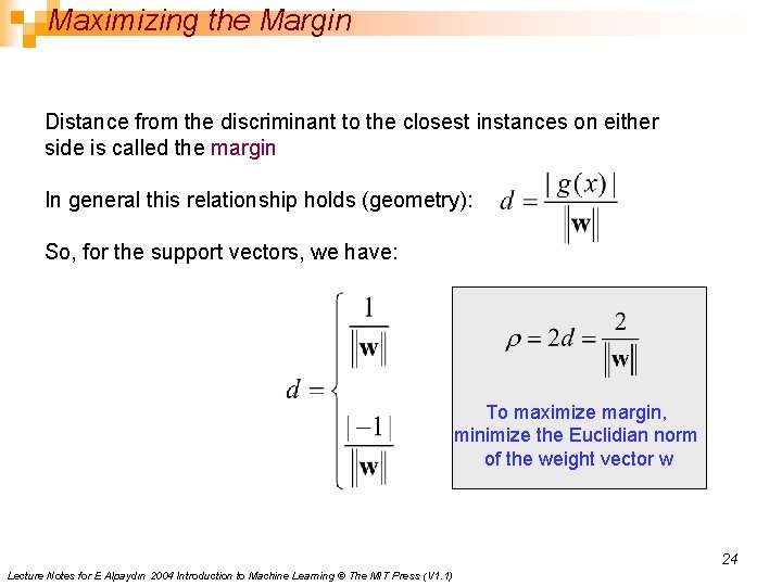
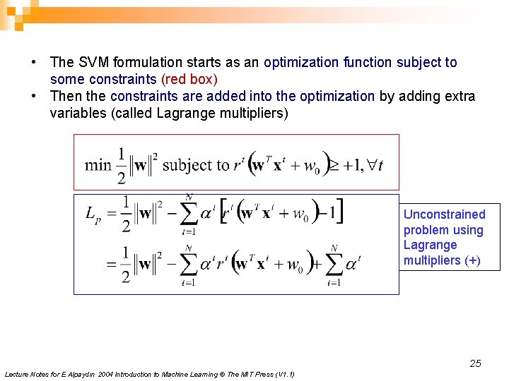
Maximizing the Margin Distance from the discriminant to the closest instances on either side is called the margin In general this relationship holds (geometry): So, for the support vectors, we have: To maximize margin, minimize the Euclidian norm of the weight vector w 24 Lecture Notes for E Alpaydın 2004 Introduction to Machine Learning © The MIT Press (V 1. 1)

• The SVM formulation starts as an optimization function subject to some constraints (red box) • Then the constraints are added into the optimization by adding extra variables (called Lagrange multipliers) Unconstrained problem using Lagrange multipliers (+) 25 Lecture Notes for E Alpaydın 2004 Introduction to Machine Learning © The MIT Press (V 1. 1)

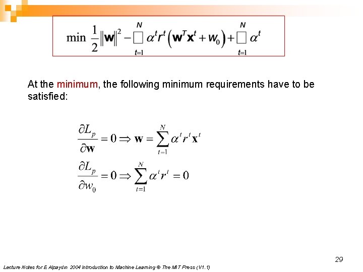
At the minimum, the following minimum requirements have to be satisfied: 29 Lecture Notes for E Alpaydın 2004 Introduction to Machine Learning © The MIT Press (V 1. 1)

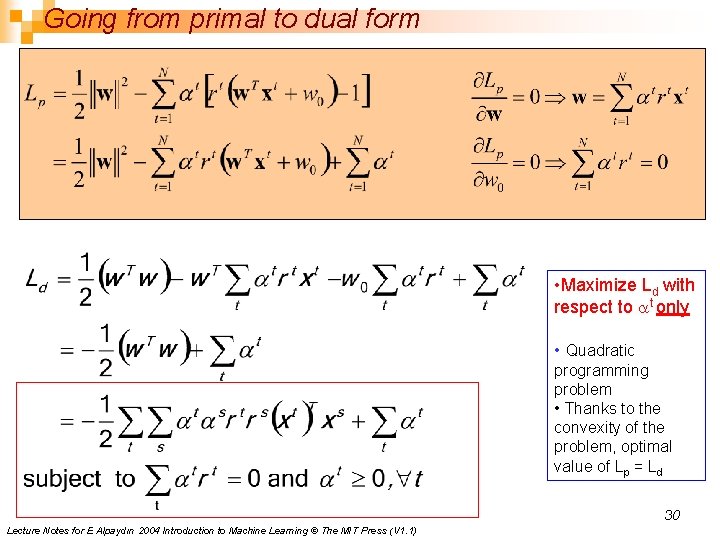
Going from primal to dual form • Maximize Ld with respect to at only • Quadratic programming problem • Thanks to the convexity of the problem, optimal value of Lp = Ld 30 Lecture Notes for E Alpaydın 2004 Introduction to Machine Learning © The MIT Press (V 1. 1)

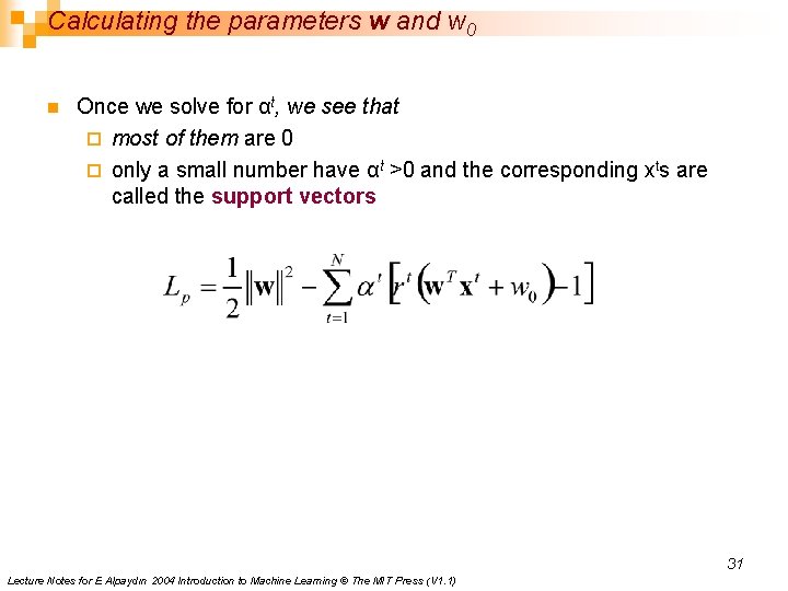
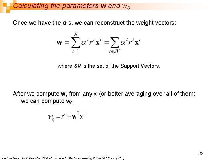
Calculating the parameters w and w 0 n Once we solve for αt, we see that ¨ most of them are 0 ¨ only a small number have αt >0 and the corresponding xts are called the support vectors 31 Lecture Notes for E Alpaydın 2004 Introduction to Machine Learning © The MIT Press (V 1. 1)

Calculating the parameters w and w 0 Once we have the αt s, we can reconstruct the weight vectors: where SV is the set of the Support Vectors. After we compute w, from any xt (or better averaging over all of them) we can compute w 0: 32 Lecture Notes for E Alpaydın 2004 Introduction to Machine Learning © The MIT Press (V 1. 1)

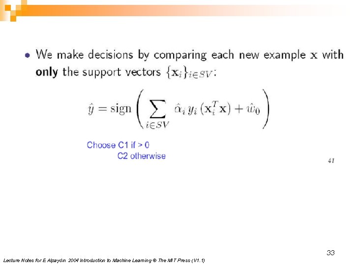
33 Lecture Notes for E Alpaydın 2004 Introduction to Machine Learning © The MIT Press (V 1. 1)

Not-Linearly Separable Case

n The non-separable case cannot find a feasible solution using the previous approach ¨ n The objective function (LD) grows arbitrarily large. Relax the constraints, but only when necessary ¨ Introduce a further cost for this 35 Lecture Notes for E Alpaydın 2004 Introduction to Machine Learning © The MIT Press (V 1. 1)

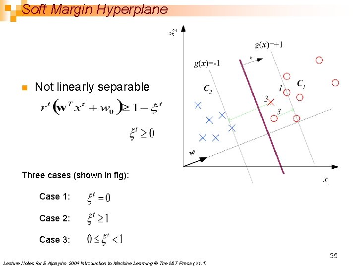
Soft Margin Hyperplane n Not linearly separable Three cases (shown in fig): Case 1: Case 2: Case 3: 36 Lecture Notes for E Alpaydın 2004 Introduction to Machine Learning © The MIT Press (V 1. 1)

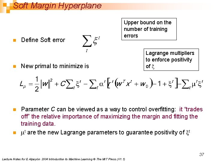
Soft Margin Hyperplane n Define Soft error Upper bound on the number of training errors Lagrange multipliers to enforce positivity of x n New primal to minimize is n Parameter C can be viewed as a way to control overfitting: it “trades off” the relative importance of maximizing the margin and fitting the training data. mt are the new Lagrange parameters to guarantee positivity of xt n 37 Lecture Notes for E Alpaydın 2004 Introduction to Machine Learning © The MIT Press (V 1. 1)

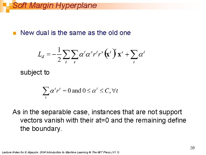
Soft Margin Hyperplane n New dual is the same as the old one subject to As in the separable case, instances that are not support vectors vanish with their at=0 and the remaining define the boundary. 38 Lecture Notes for E Alpaydın 2004 Introduction to Machine Learning © The MIT Press (V 1. 1)

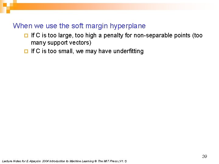
When we use the soft margin hyperplane If C is too large, too high a penalty for non-separable points (too many support vectors) ¨ If C is too small, we may have underfitting ¨ 39 Lecture Notes for E Alpaydın 2004 Introduction to Machine Learning © The MIT Press (V 1. 1)

Kernel Functions in SVM

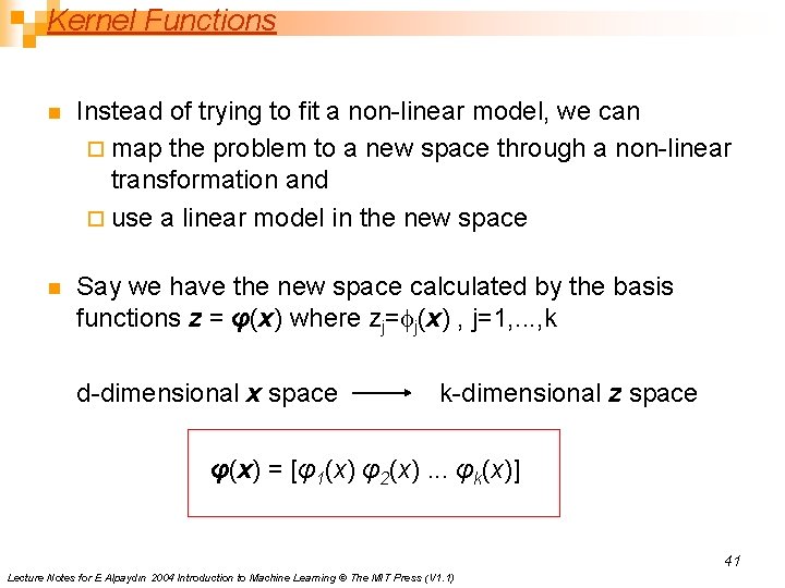
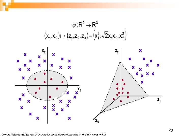
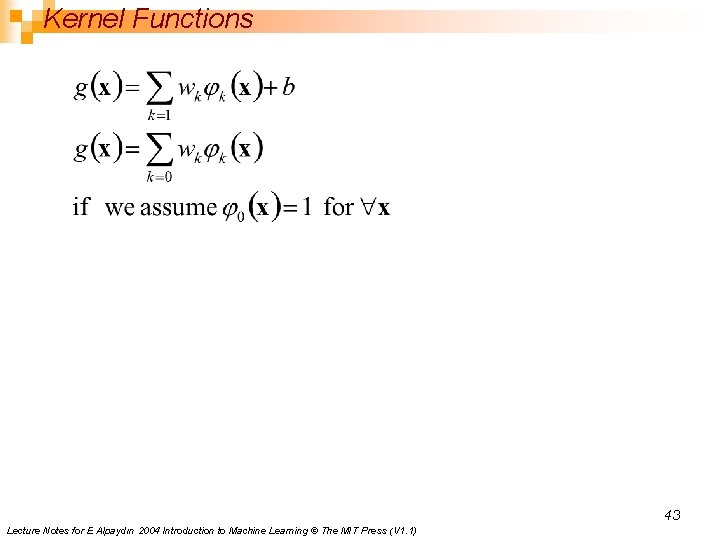
Kernel Functions n Instead of trying to fit a non-linear model, we can ¨ map the problem to a new space through a non-linear transformation and ¨ use a linear model in the new space n Say we have the new space calculated by the basis functions z = φ(x) where zj=fj(x) , j=1, . . . , k d-dimensional x space k-dimensional z space φ(x) = [φ1(x) φ2(x). . . φk(x)] 41 Lecture Notes for E Alpaydın 2004 Introduction to Machine Learning © The MIT Press (V 1. 1)

42 Lecture Notes for E Alpaydın 2004 Introduction to Machine Learning © The MIT Press (V 1. 1)

Kernel Functions 43 Lecture Notes for E Alpaydın 2004 Introduction to Machine Learning © The MIT Press (V 1. 1)

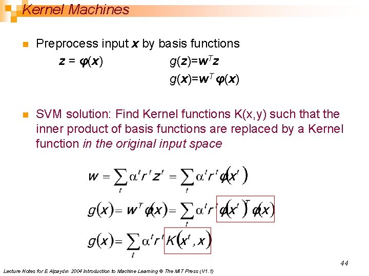
Kernel Machines n Preprocess input x by basis functions z = φ(x) g(z)=w. Tz g(x)=w. T φ(x) n SVM solution: Find Kernel functions K(x, y) such that the inner product of basis functions are replaced by a Kernel function in the original input space 44 Lecture Notes for E Alpaydın 2004 Introduction to Machine Learning © The MIT Press (V 1. 1)

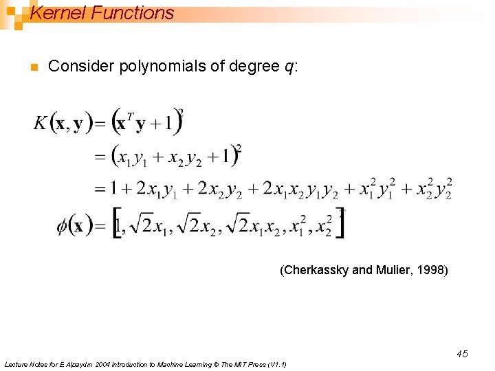
Kernel Functions n Consider polynomials of degree q: (Cherkassky and Mulier, 1998) 45 Lecture Notes for E Alpaydın 2004 Introduction to Machine Learning © The MIT Press (V 1. 1)

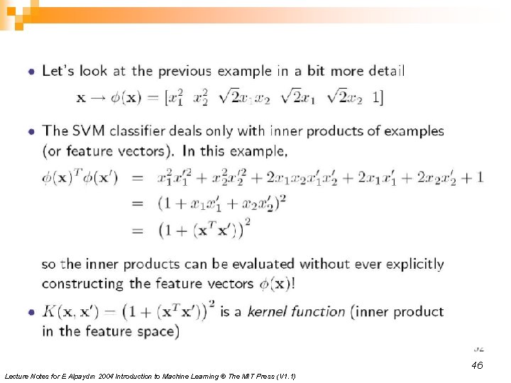
46 Lecture Notes for E Alpaydın 2004 Introduction to Machine Learning © The MIT Press (V 1. 1)

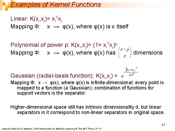
Examples of Kernel Functions Linear: K(xi, xj)= xi. Txj Mapping Φ: x → φ(x), where φ(x) is x itself Polynomial of power p: K(xi, xj)= (1+ xi. Txj)p Mapping Φ: x → φ(x), where φ(x) has dimensions Gaussian (radial-basis function): K(xi, xj) = Mapping Φ: x → φ(x), where φ(x) is infinite-dimensional: every point is mapped to a function (a Gaussian); combination of functions for support vectors is the separator. Higher-dimensional space still has intrinsic dimensionality d, but linear separators in it correspond to non-linear separators in original space. 47 Lecture Notes for E Alpaydın 2004 Introduction to Machine Learning © The MIT Press (V 1. 1)

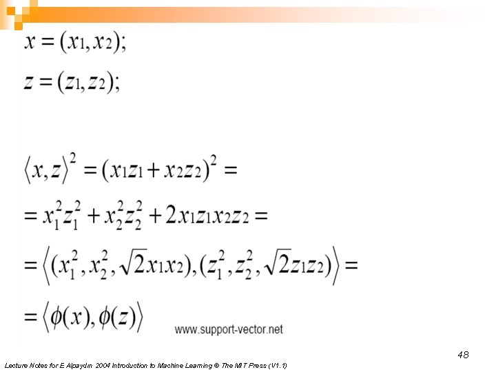
48 Lecture Notes for E Alpaydın 2004 Introduction to Machine Learning © The MIT Press (V 1. 1)

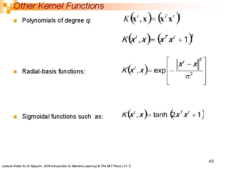
Other Kernel Functions n Polynomials of degree q: n Radial-basis functions: n Sigmoidal functions such as: 49 Lecture Notes for E Alpaydın 2004 Introduction to Machine Learning © The MIT Press (V 1. 1)

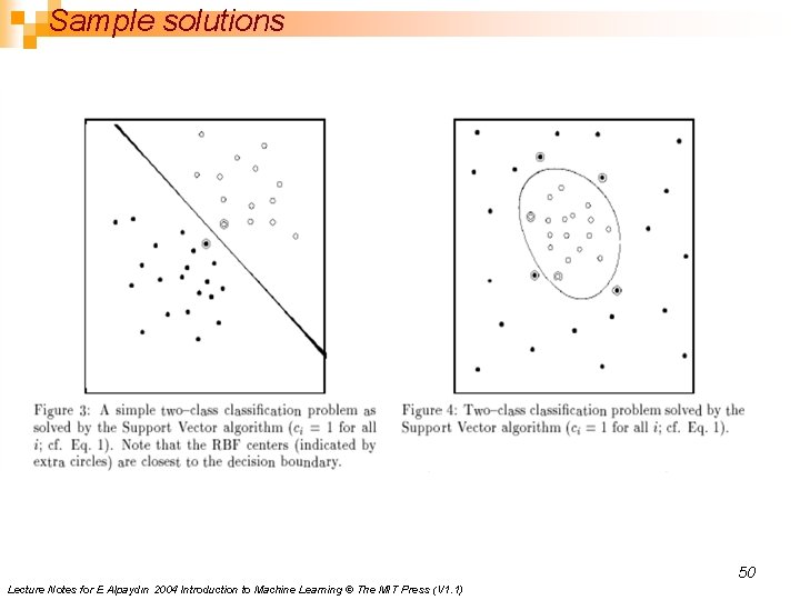
Sample solutions 50 Lecture Notes for E Alpaydın 2004 Introduction to Machine Learning © The MIT Press (V 1. 1)

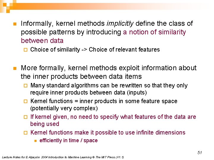
n Informally, kernel methods implicitly define the class of possible patterns by introducing a notion of similarity between data ¨ n Choice of similarity -> Choice of relevant features More formally, kernel methods exploit information about the inner products between data items Many standard algorithms can be rewritten so that they only require inner products between data (inputs) ¨ Kernel functions = inner products in some feature space (potentially very complex) ¨ If kernel given, no need to specify what features of the data are being used ¨ Kernel functions make it possible to use infinite dimensions ¨ n efficiently in time / space 51 Lecture Notes for E Alpaydın 2004 Introduction to Machine Learning © The MIT Press (V 1. 1)

SVM summary n SVMs were originally proposed by Boser, Guyon and Vapnik in 1992 and gained increasing popularity in late 1990 s. n SVMs represent a general methodology for many PR problems: classification, regression, feature extraction, clustering, novelty detection, etc. n SVMs can be applied to complex data types beyond feature vectors (e. g. graphs, sequences, relational data) by designing kernel functions for such data. n SVM techniques have been extended to a number of tasks such as regression [Vapnik et al. ’ 97], principal component analysis [Schölkopf et al. ’ 99], etc. n Most popular optimization algorithms for SVMs use decomposition to hillclimb over a subset of αi’s at a time, e. g. SMO [Platt ’ 99] and [Joachims ’ 99] 52 Lecture Notes for E Alpaydın 2004 Introduction to Machine Learning © The MIT Press (V 1. 1)

Advantages of SVMs ¨ There are no problems with local minima, because the solution is a Qaudratic Programming problem ¨ The optimal solution can be found in polynomial time ¨ There are few model parameters to select: the penalty term C, the kernel function and parameters (e. g. , spread σ in the case of RBF kernels) ¨ The final results are stable and repeatable (e. g. , no random initial weights) ¨ The SVM solution is sparse; it only involves the support vectors ¨ SVMs rely on elegant and principled learning methods ¨ SVMs provide a method to control complexity independently of dimensionality ¨ SVMs have been shown (theoretically and empirically) to have excellent generalization capabilities 53 Lecture Notes for E Alpaydın 2004 Introduction to Machine Learning © The MIT Press (V 1. 1)

Challenges n Can the kernel functions be selected in a principled manner? n SVMs still require selection of a few parameters, typically through cross-validation n How does one incorporate domain knowledge? ¨ Currently this is performed through the selection of the kernel and the introduction of “artificial” examples n How interpretable are the results provided by an SVM? n What is the optimal data representation for SVM? What is the effect of feature weighting? How does an SVM handle categorical or missing features? n Do SVMs always perform best? Can they beat a hand-crafted solution for a particular problem? n Do SVMs eliminate the model selection problem? 54 Lecture Notes for E Alpaydın 2004 Introduction to Machine Learning © The MIT Press (V 1. 1)

n More explanations or demonstrations can be found at: ¨ ¨ ¨ http: //www. support-vector-machines. org/index. html Haykin Chp. 6 pp. 318 -339 Burges tutorial (under/reading/) n ¨ n n http: //www. dtreg. com/svm. htm Software ¨ SVMlight, by Joachims, is one of the most widely used SVM classification and regression package. Distributed as C++ source and binaries for Linux, Windows, Cygwin, and Solaris. Kernels: polynomial, radial basis function, and neural (tanh). ¨ Lib. SVM http: //www. csie. ntu. edu. tw/~cjlin/libsvm/ LIBSVM (Library for Support Vector Machines), is developed by Chang and Lin; also widely used. Developed in C++ and Java, it supports also multi-classification, weighted SVM for unbalanced data, cross-validation and automatic model selection. It has interfaces for Python, R, Splus, MATLAB, Perl, Ruby, and Lab. VIEW. Kernels: linear, polynomial, radial basis function, and neural (tanh). Applet to play with: ¨ n Burges, CJC "A Tutorial on Support Vector Machines for Pattern Recognition" Data Mining and Knowledge Discovery, Vol 2 No 2, 1998. http: //lcn. epfl. ch/tutorial/english/svm/html/index. html Some non-SVM good applets: ¨ http: //cs. stanford. edu/people/karpathy/convnetjs/ Lecture Notes for E Alpaydın 2004 Introduction to Machine Learning © The MIT Press (V 1. 1) 55

SVM Applications n Cortes and Vapnik 1995: ¨ ¨ ¨ Handwritten digit classification 16 x 16 bitmaps -> 256 dimensions Polynomial kernel where q=3 -> feature space with 106 dimensions No overfitting on a training set of 7300 instances Average of 148 support vectors over different training sets Expected test error rate: Exp. N[P(error)] = Exp. N[#support vectors] / N (= 0. 02 for the above example) 56 Lecture Notes for E Alpaydın 2004 Introduction to Machine Learning © The MIT Press (V 1. 1)

n The main things to know are: ¨ ¨ ¨ The aim of SVMs (maximizing the margins) How it is specified as an optimization problem Once solved, the optimization finds the as, that in turn specifies the weights n as also indicate which input data are the support vectors (those for which the corresponding a is non-zero) The non-linearly separable case can be handled in a similar manner, with a slight extension that involves a parameter C n It is important to understand what C does in order to properly use SVM software The use of kernels makes it possible to go to higher dimensional space, without actually computing those features explicitly; nor being badly affected by the curse of dimensionality 57 Lecture Notes for E Alpaydın 2004 Introduction to Machine Learning © The MIT Press (V 1. 1)