Lecture Slides for INTRODUCTION TO Machine Learning ETHEM

Lecture Slides for INTRODUCTION TO Machine Learning ETHEM ALPAYDIN © The MIT Press, 2010 alpaydin@boun. edu. tr http: //www. cmpe. boun. edu. tr/~ethem/i 2 ml 2 e

CHAPTER 2: Supervised Learning

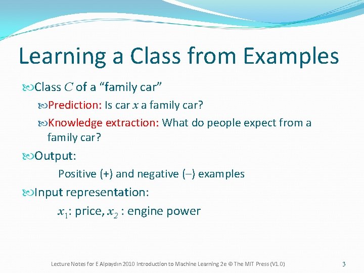
Learning a Class from Examples Class C of a “family car” Prediction: Is car x a family car? Knowledge extraction: What do people expect from a family car? Output: Positive (+) and negative (–) examples Input representation: x 1: price, x 2 : engine power Lecture Notes for E Alpaydın 2010 Introduction to Machine Learning 2 e © The MIT Press (V 1. 0) 3

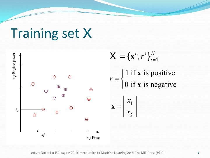
Training set X Lecture Notes for E Alpaydın 2010 Introduction to Machine Learning 2 e © The MIT Press (V 1. 0) 4

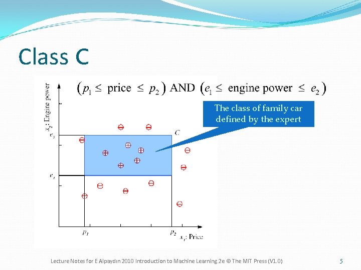
Class C The class of family car defined by the expert Lecture Notes for E Alpaydın 2010 Introduction to Machine Learning 2 e © The MIT Press (V 1. 0) 5

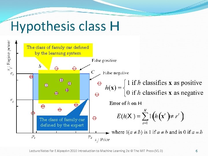
Hypothesis class H The class of family car defined by the learning system Error of h on H The class of family car defined by the expert Lecture Notes for E Alpaydın 2010 Introduction to Machine Learning 2 e © The MIT Press (V 1. 0) 6

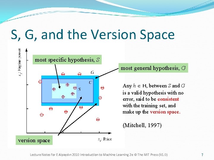
S, G, and the Version Space most specific hypothesis, S most general hypothesis, G Any h Î H, between S and G is a valid hypothesis with no error, said to be consistent with the training set, and make up the version space. (Mitchell, 1997) version space Lecture Notes for E Alpaydın 2010 Introduction to Machine Learning 2 e © The MIT Press (V 1. 0) 7

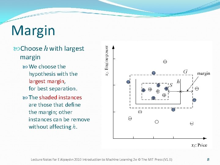
Margin Choose h with largest margin We choose the hypothesis with the largest margin, for best separation. The shaded instances are those that define the margin; other instances can be remove without affecting h. Lecture Notes for E Alpaydın 2010 Introduction to Machine Learning 2 e © The MIT Press (V 1. 0) 8

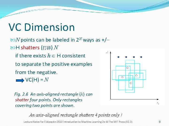
VC Dimension N points can be labeled in 2 N ways as +/– H shatters (打碎) N if there exists h Î H consistent to separate the positive examples from the negative. VC(H) = N Fig. 2. 6 An axis-aligned rectangle (h) can shatter four points. Only rectangles covering two points are shown. An axis-aligned rectangle shatters 4 points only ! Lecture Notes for E Alpaydın 2010 Introduction to Machine Learning 2 e © The MIT Press (V 1. 0) 9

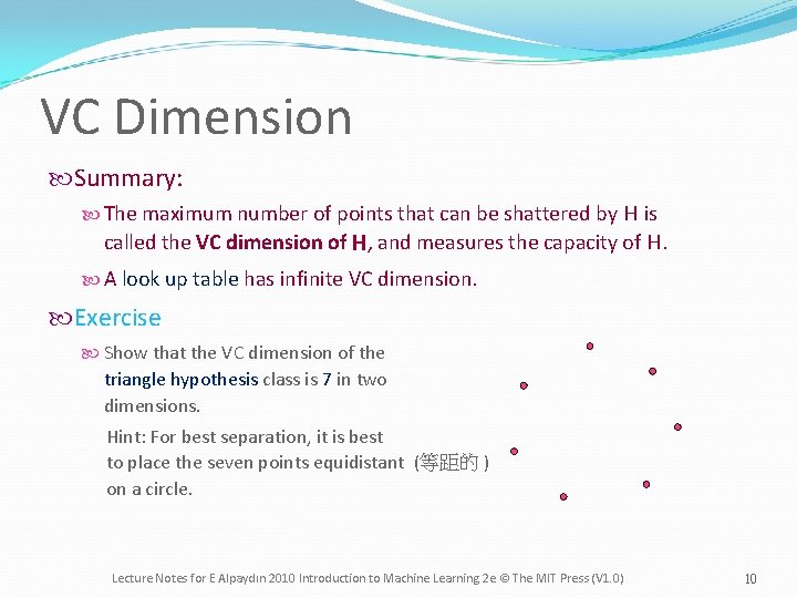
VC Dimension Summary: The maximum number of points that can be shattered by H is called the VC dimension of H, and measures the capacity of H. A look up table has infinite VC dimension. Exercise Show that the VC dimension of the triangle hypothesis class is 7 in two dimensions. Hint: For best separation, it is best to place the seven points equidistant (等距的 ) on a circle. Lecture Notes for E Alpaydın 2010 Introduction to Machine Learning 2 e © The MIT Press (V 1. 0) 10

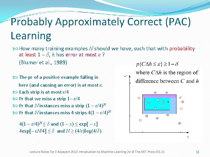
Probably Approximately Correct (PAC) Learning How many training examples N should we have, such that with probability at least 1 ‒ δ, h has error at most ε ? (Blumer et al. , 1989) The pr of a positive example falling in here (and causing an error) is at most ε. Each strip is at most ε/4 Pr that we miss a strip 1‒ ε/4 Pr that N instances miss a strip (1 ‒ ε/4)N Pr that N instances miss 4 strips 4(1 ‒ ε/4)N ≤ δ and (1 ‒ x) ≤ exp[ ‒ x] 4 exp[‒ εN/4] ≤ δ and N ≥ (4/ε)log(4/δ) Lecture Notes for E Alpaydın 2010 Introduction to Machine Learning 2 e © The MIT Press (V 1. 0) 11

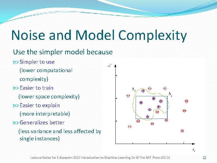
Noise and Model Complexity Use the simpler model because Simpler to use (lower computational complexity) Easier to train (lower space complexity) Easier to explain (more interpretable) Generalizes better (less variance and less affected by single instances) Lecture Notes for E Alpaydın 2010 Introduction to Machine Learning 2 e © The MIT Press (V 1. 0) 12

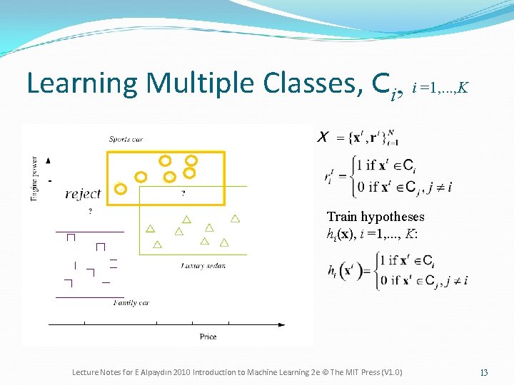
Learning Multiple Classes, Ci, i =1, . . . , K Train hypotheses hi(x), i =1, . . . , K: Lecture Notes for E Alpaydın 2010 Introduction to Machine Learning 2 e © The MIT Press (V 1. 0) 13

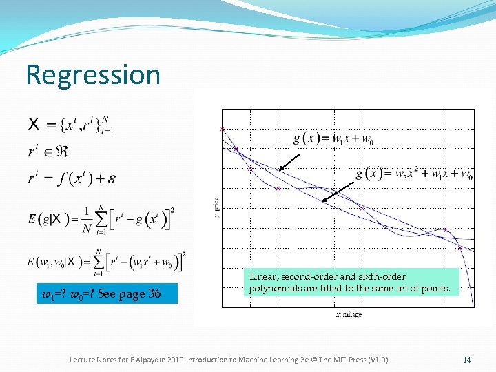
Regression w 1=? w 0=? See page 36 Linear, second-order and sixth-order polynomials are fitted to the same set of points. Lecture Notes for E Alpaydın 2010 Introduction to Machine Learning 2 e © The MIT Press (V 1. 0) 14

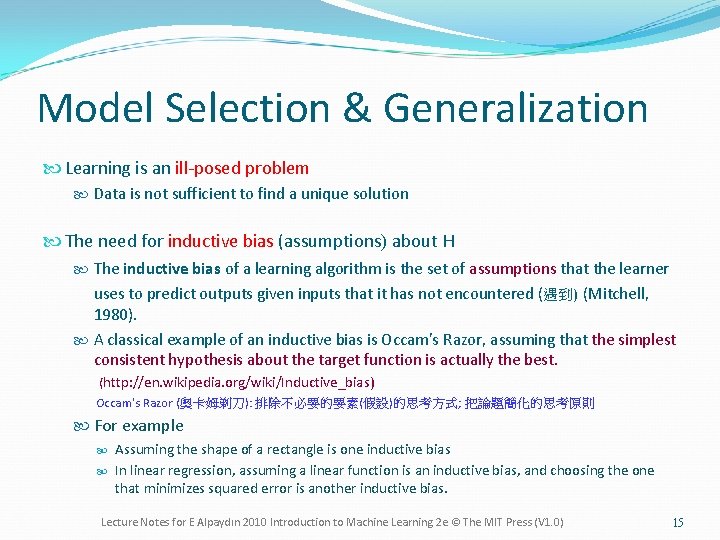
Model Selection & Generalization Learning is an ill-posed problem Data is not sufficient to find a unique solution The need for inductive bias (assumptions) about H The inductive bias of a learning algorithm is the set of assumptions that the learner uses to predict outputs given inputs that it has not encountered (遇到) (Mitchell, 1980). A classical example of an inductive bias is Occam's Razor, assuming that the simplest consistent hypothesis about the target function is actually the best. (http: //en. wikipedia. org/wiki/Inductive_bias) Occam's Razor (奧卡姆剃刀): 排除不必要的要素(假設)的思考方式; 把論題簡化的思考原則 For example Assuming the shape of a rectangle is one inductive bias In linear regression, assuming a linear function is an inductive bias, and choosing the one that minimizes squared error is another inductive bias. Lecture Notes for E Alpaydın 2010 Introduction to Machine Learning 2 e © The MIT Press (V 1. 0) 15

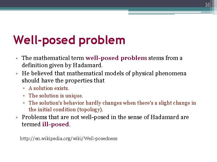
16 Well-posed problem • The mathematical term well-posed problem stems from a definition given by Hadamard. • He believed that mathematical models of physical phenomena should have the properties that ▫ A solution exists. ▫ The solution is unique. ▫ The solution's behavior hardly changes when there's a slight change in the initial condition (topology). • Problems that are not well-posed in the sense of Hadamard are termed ill-posed. http: //en. wikipedia. org/wiki/Well-posedness

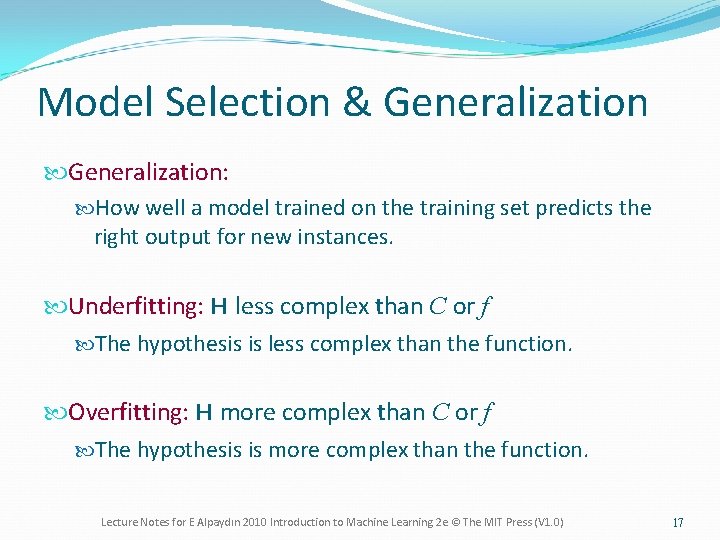
Model Selection & Generalization: How well a model trained on the training set predicts the right output for new instances. Underfitting: H less complex than C or f The hypothesis is less complex than the function. Overfitting: H more complex than C or f The hypothesis is more complex than the function. Lecture Notes for E Alpaydın 2010 Introduction to Machine Learning 2 e © The MIT Press (V 1. 0) 17

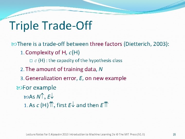
Triple Trade-Off There is a trade-off between three factors (Dietterich, 2003): 1. Complexity of H, c(H) ¨ c (H) : the capacity of the hypothesis class 2. The amount of training data, N 3. Generalization error, E, on new example For example As N , E¯ 1. As c (H) , first E¯ and then E Lecture Notes for E Alpaydın 2010 Introduction to Machine Learning 2 e © The MIT Press (V 1. 0) 18

19 Cross-Validation • Cross-validation is the statistical practice of partitioning a sample of data into subsets such that the analysis is initially performed on a single subset, while the other subset(s) are retained (保留) for subsequent (隨後的) use in confirming and validating (證實) the initial analysis. (http: //en. wikipedia. org/wiki/Cross-validation)

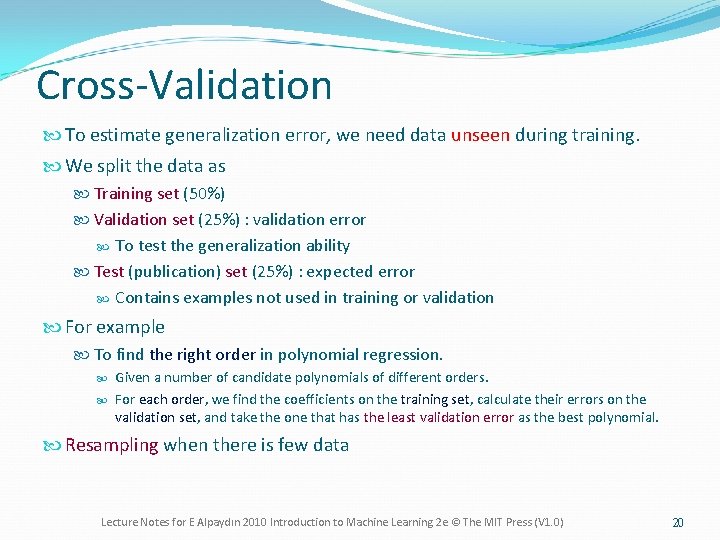
Cross-Validation To estimate generalization error, we need data unseen during training. We split the data as Training set (50%) Validation set (25%) : validation error To test the generalization ability Test (publication) set (25%) : expected error Contains examples not used in training or validation For example To find the right order in polynomial regression. Given a number of candidate polynomials of different orders. For each order, we find the coefficients on the training set, calculate their errors on the validation set, and take the one that has the least validation error as the best polynomial. Resampling when there is few data Lecture Notes for E Alpaydın 2010 Introduction to Machine Learning 2 e © The MIT Press (V 1. 0) 20

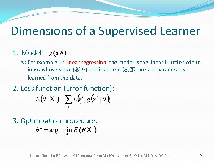
Dimensions of a Supervised Learner 1. Model: For example, in linear regression, the model is the linear function of the input whose slope (斜率) and intercept (截距) are the parameters learned from the data. 2. Loss function (Error function): 3. Optimization procedure: Lecture Notes for E Alpaydın 2010 Introduction to Machine Learning 2 e © The MIT Press (V 1. 0) 21

Exercise The complexity of most learning algorithms is a function of the training set. Can you proposed a filtering algorithm that finds redundant instances? If we have a supervisor who can provide us with the label for any x, where should we choose x to learn with fewer queries? Lecture Notes for E Alpaydın 2010 Introduction to Machine Learning 2 e © The MIT Press (V 1. 0) 22