Lecture Slides for INTRODUCTION TO Machine Learning ETHEM
- Slides: 23

Lecture Slides for INTRODUCTION TO Machine Learning ETHEM ALPAYDIN © The MIT Press, 2004 alpaydin@boun. edu. tr http: //www. cmpe. boun. edu. tr/~ethem/i 2 ml

Outline n Discriminant Function n Learning Association Rules n Naïve Bayes Classifier n Example: Play Tennis n Relevant Issues n Conclusions 2

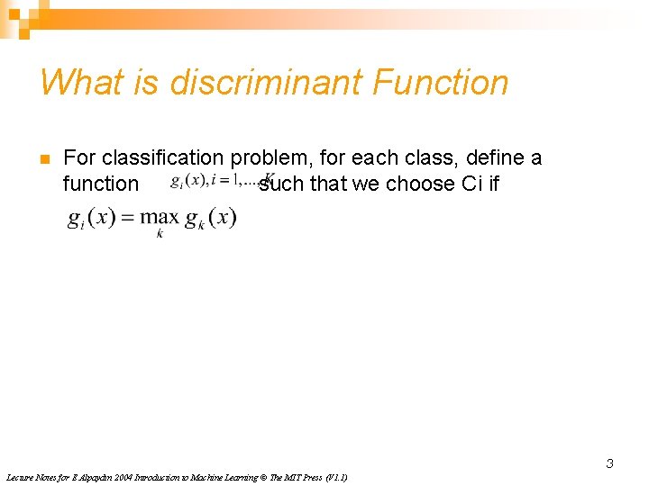
What is discriminant Function n For classification problem, for each class, define a function such that we choose Ci if 3 Lecture Notes for E Alpaydın 2004 Introduction to Machine Learning © The MIT Press (V 1. 1)

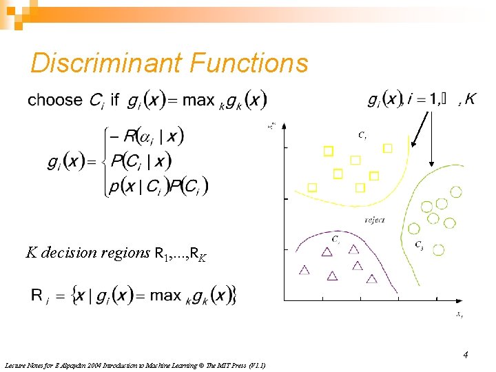
Discriminant Functions K decision regions R 1, . . . , RK 4 Lecture Notes for E Alpaydın 2004 Introduction to Machine Learning © The MIT Press (V 1. 1)

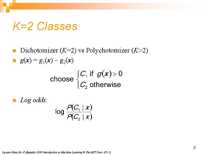
K=2 Classes n Dichotomizer (K=2) vs Polychotomizer (K>2) g(x) = g 1(x) – g 2(x) n Log odds: n 5 Lecture Notes for E Alpaydın 2004 Introduction to Machine Learning © The MIT Press (V 1. 1)

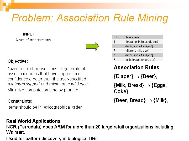
Problem: Association Rule Mining INPUT A set of transactions Objective: Given a set of transactions D, generate all association rules that have support and confidence greater than the user-specified minimum support and minimum confidence. Minimize computation time by pruning. Constraints: Items should be in lexicographical order Association Rules {Diaper} {Beer}, {Milk, Bread} {Eggs, Coke}, {Beer, Bread} {Milk}, Real World Applications NCR (Terradata) does ARM for more than 20 large retail organizations including Walmart. Used for pattern discovery in biological DBs.

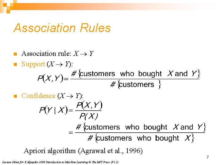
Association Rules n Association rule: X Y Support (X Y): n Confidence (X Y): n Apriori algorithm (Agrawal et al. , 1996) 7 Lecture Notes for E Alpaydın 2004 Introduction to Machine Learning © The MIT Press (V 1. 1)

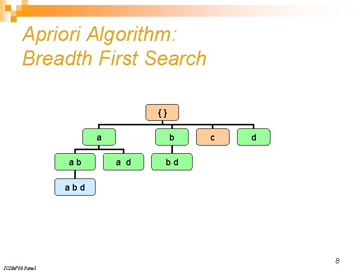
Apriori Algorithm: Breadth First Search {} a ab b a d c d bd abd 8 ICDM'06 Panel

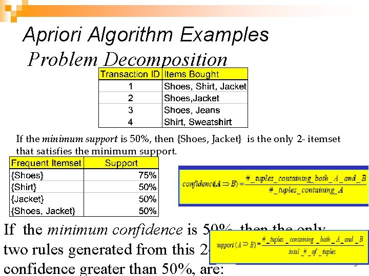
Apriori Algorithm Examples Problem Decomposition If the minimum support is 50%, then {Shoes, Jacket} is the only 2 - itemset that satisfies the minimum support. If the minimum confidence is 50%, then the only two rules generated from this 2 -itemset, that have confidence greater than 50%, are: 9

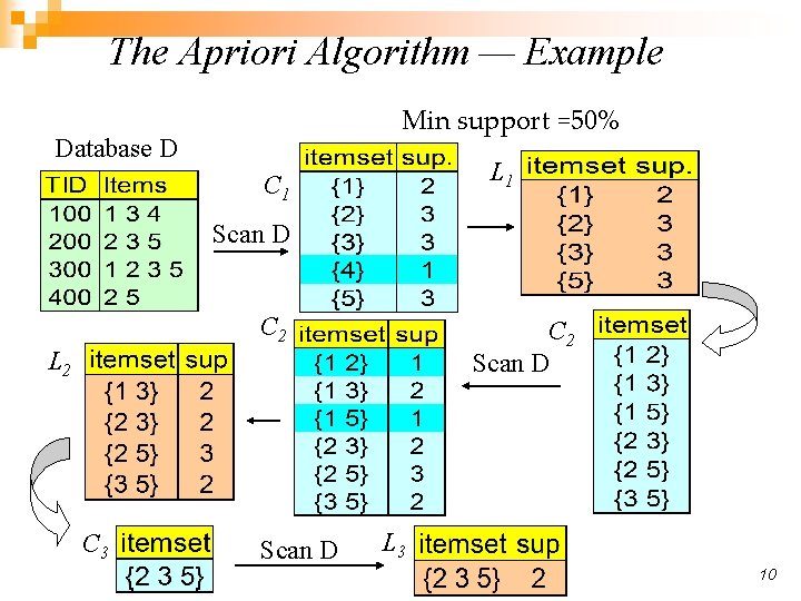
The Apriori Algorithm — Example Min support =50% Database D L 1 C 1 Scan D C 2 Scan D L 2 C 3 Scan D L 3 10

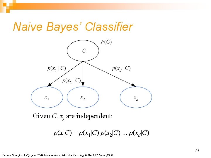
Naive Bayes’ Classifier Given C, xj are independent: p(x|C) = p(x 1|C) p(x 2|C). . . p(xd|C) 11 Lecture Notes for E Alpaydın 2004 Introduction to Machine Learning © The MIT Press (V 1. 1)

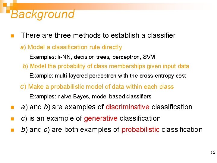
Background n There are three methods to establish a classifier a) Model a classification rule directly Examples: k-NN, decision trees, perceptron, SVM b) Model the probability of class memberships given input data Example: multi-layered perceptron with the cross-entropy cost c) Make a probabilistic model of data within each class Examples: naive Bayes, model based classifiers n a) and b) are examples of discriminative classification n c) is an example of generative classification n b) and c) are both examples of probabilistic classification 12

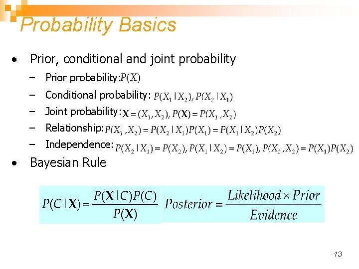
Probability Basics • Prior, conditional and joint probability – Prior probability: – Conditional probability: – Joint probability: – Relationship: – Independence: • Bayesian Rule 13

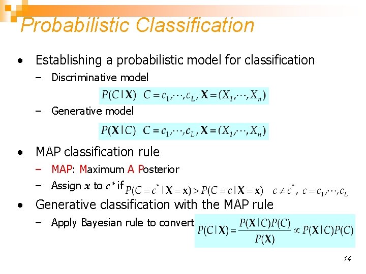
Probabilistic Classification • Establishing a probabilistic model for classification – Discriminative model – Generative model • MAP classification rule – MAP: Maximum A Posterior – Assign x to c* if • Generative classification with the MAP rule – Apply Bayesian rule to convert: 14

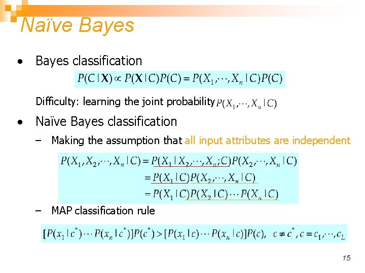
Naïve Bayes • Bayes classification Difficulty: learning the joint probability • Naïve Bayes classification – Making the assumption that all input attributes are independent – MAP classification rule 15

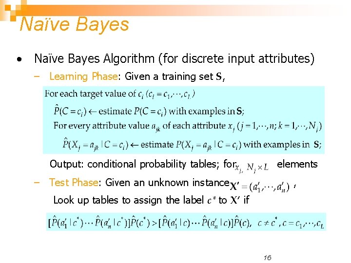
Naïve Bayes • Naïve Bayes Algorithm (for discrete input attributes) – Learning Phase: Given a training set S, Output: conditional probability tables; for elements – Test Phase: Given an unknown instance , Look up tables to assign the label c* to X’ if 16

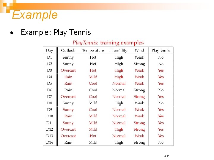
Example • Example: Play Tennis 17

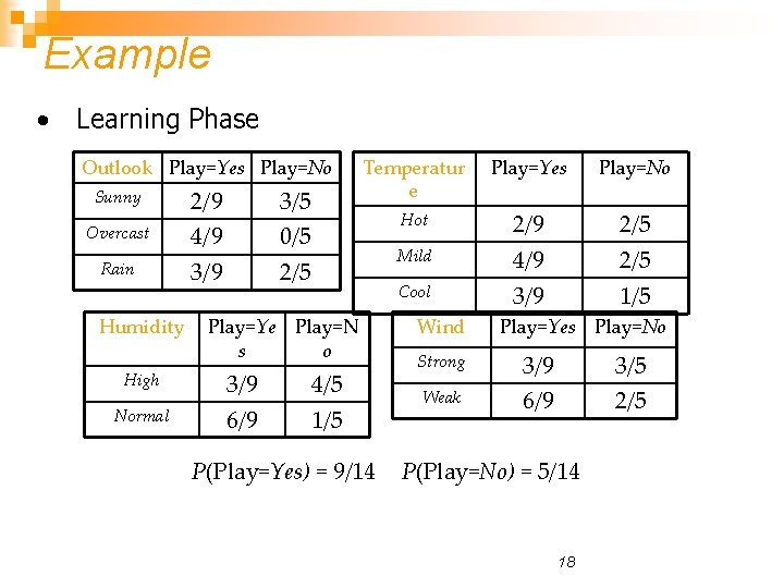
Example • Learning Phase Outlook Play=Yes Play=No Sunny Overcast Rain Humidity High Normal 2/9 4/9 3/5 0/5 2/5 Temperatur e Play=Yes Play=No Hot 2/9 4/9 3/9 2/5 1/5 Mild Cool Play=Ye Play=N s o 3/9 6/9 4/5 1/5 P(Play=Yes) = 9/14 Wind Strong Weak Play=Yes Play=No 3/9 6/9 3/5 2/5 P(Play=No) = 5/14 18

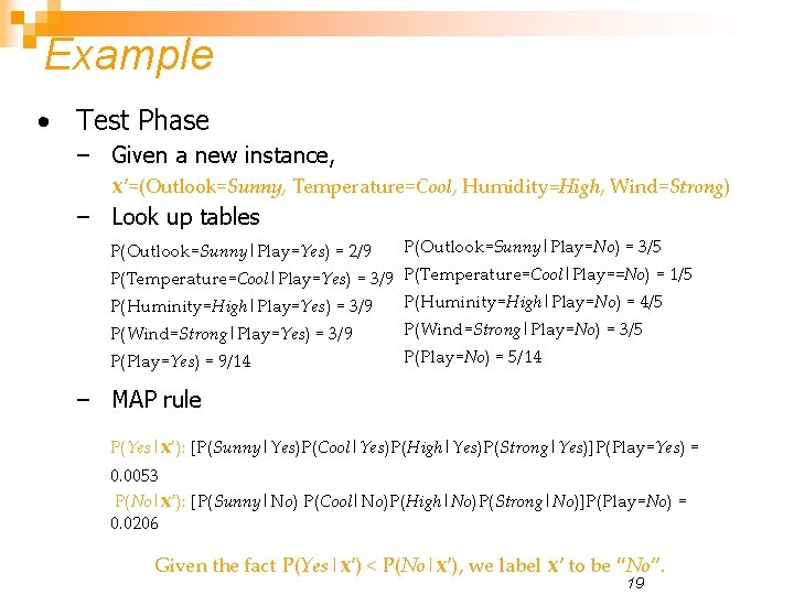
Example • Test Phase – Given a new instance, x’=(Outlook=Sunny, Temperature=Cool, Humidity=High, Wind=Strong) – Look up tables P(Outlook=Sunny|Play=Yes) = 2/9 P(Outlook=Sunny|Play=No) = 3/5 P(Wind=Strong|Play=Yes) = 3/9 P(Wind=Strong|Play=No) = 3/5 P(Temperature=Cool|Play=Yes) = 3/9 P(Temperature=Cool|Play==No) = 1/5 P(Huminity=High|Play=No) = 4/5 P(Huminity=High|Play=Yes) = 3/9 P(Play=Yes) = 9/14 P(Play=No) = 5/14 – MAP rule P(Yes|x’): [P(Sunny|Yes)P(Cool|Yes)P(High|Yes)P(Strong|Yes)]P(Play=Yes) = 0. 0053 P(No|x’): [P(Sunny|No) P(Cool|No)P(High|No)P(Strong|No)]P(Play=No) = 0. 0206 Given the fact P(Yes|x’) < P(No|x’), we label x’ to be “No”. 19

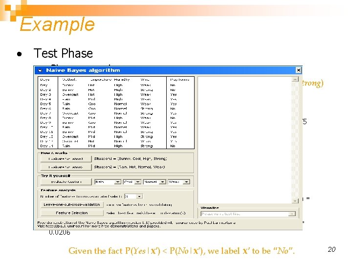
Example • Test Phase – Given a new instance, x’=(Outlook=Sunny, Temperature=Cool, Humidity=High, Wind=Strong) – Look up tables P(Outlook=Sunny|Play=Yes) = 2/9 P(Outlook=Sunny|Play=No) = 3/5 P(Wind=Strong|Play=Yes) = 3/9 P(Wind=Strong|Play=No) = 3/5 P(Temperature=Cool|Play=Yes) = 3/9 P(Temperature=Cool|Play==No) = 1/5 P(Huminity=High|Play=No) = 4/5 P(Huminity=High|Play=Yes) = 3/9 P(Play=Yes) = 9/14 P(Play=No) = 5/14 – MAP rule P(Yes|x’): [P(Sunny|Yes)P(Cool|Yes)P(High|Yes)P(Strong|Yes)]P(Play=Yes) = 0. 0053 P(No|x’): [P(Sunny|No) P(Cool|No)P(High|No)P(Strong|No)]P(Play=No) = 0. 0206 Given the fact P(Yes|x’) < P(No|x’), we label x’ to be “No”. 20

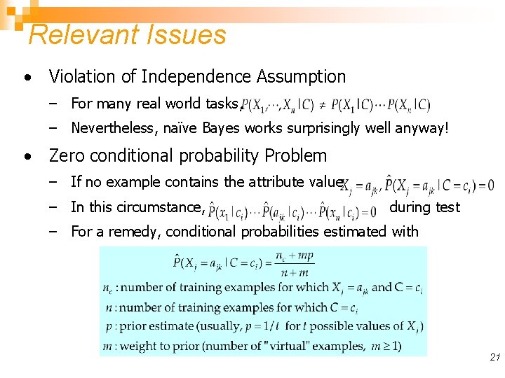
Relevant Issues • Violation of Independence Assumption – For many real world tasks, – Nevertheless, naïve Bayes works surprisingly well anyway! • Zero conditional probability Problem – If no example contains the attribute value – In this circumstance, during test – For a remedy, conditional probabilities estimated with 21

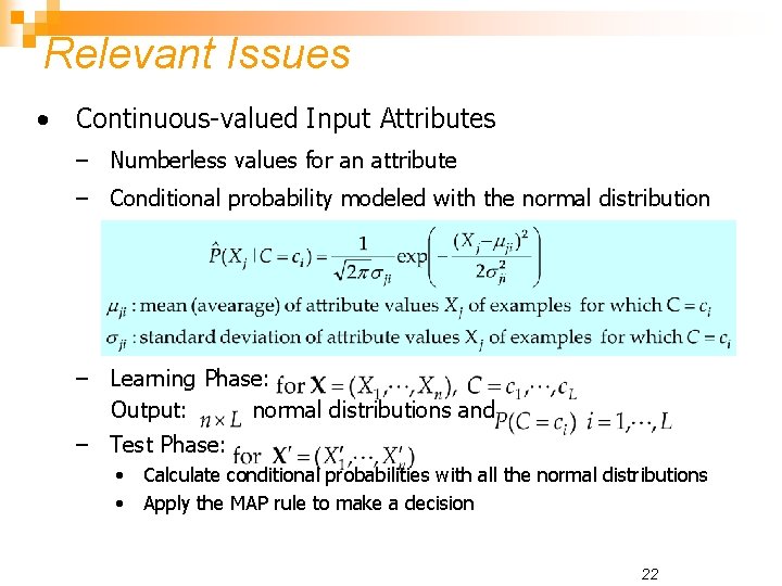
Relevant Issues • Continuous-valued Input Attributes – Numberless values for an attribute – Conditional probability modeled with the normal distribution – Learning Phase: Output: normal distributions and – Test Phase: • Calculate conditional probabilities with all the normal distributions • Apply the MAP rule to make a decision 22

Conclusions n n Naïve Bayes based on the independence assumption ¨ Training is very easy and fast; just requiring considering each attribute in each class separately ¨ Test is straightforward; just looking up tables or calculating conditional probabilities with normal distributions A popular generative model ¨ Performance competitive to most of state-of-the-art classifiers even in presence of violating independence assumption ¨ Many successful applications, e. g. , spam mail filtering ¨ Apart from classification, naïve Bayes can do more… 23