Lecture Slides for INTRODUCTION TO Machine Learning ETHEM

Lecture Slides for INTRODUCTION TO Machine Learning ETHEM ALPAYDIN © The MIT Press, 2004 alpaydin@boun. edu. tr http: //www. cmpe. boun. edu. tr/~ethem/i 2 ml Lecture Notes for E Alpaydın 2004 Introduction to Machine Learning © The MIT Press (V 1. 1)

CHAPTER 4: Parametric Methods Lecture Notes for E Alpaydın 2004 Introduction to Machine Learning © The MIT Press (V 1. 1)

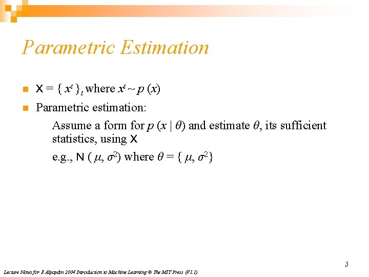
Parametric Estimation n X = { xt }t where xt ~ p (x) n Parametric estimation: Assume a form for p (x | θ) and estimate θ, its sufficient statistics, using X e. g. , N ( μ, σ2) where θ = { μ, σ2} 3 Lecture Notes for E Alpaydın 2004 Introduction to Machine Learning © The MIT Press (V 1. 1)

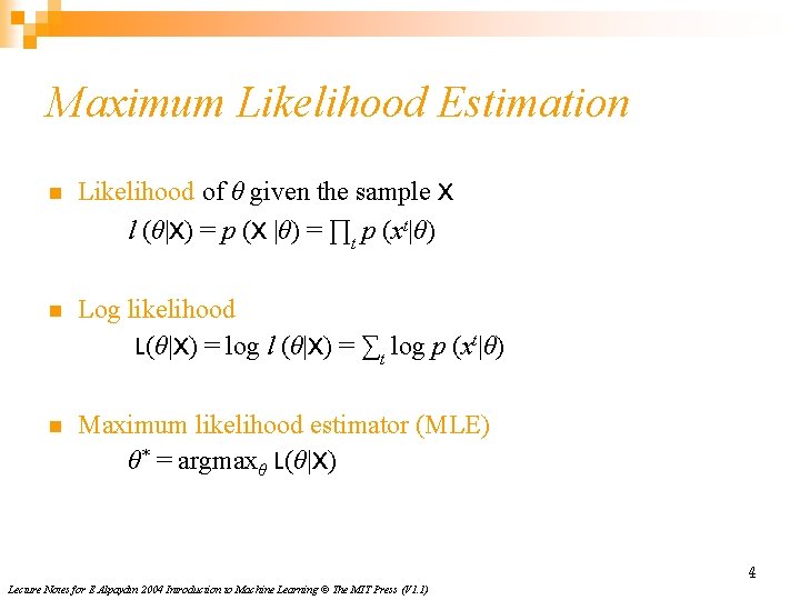
Maximum Likelihood Estimation n Likelihood of θ given the sample X l (θ|X) = p (X |θ) = ∏t p (xt|θ) n Log likelihood L(θ|X) = log l (θ|X) = ∑t log p (xt|θ) n Maximum likelihood estimator (MLE) θ* = argmaxθ L(θ|X) 4 Lecture Notes for E Alpaydın 2004 Introduction to Machine Learning © The MIT Press (V 1. 1)

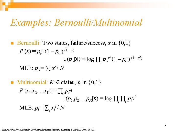
Examples: Bernoulli/Multinomial n Bernoulli: Two states, failure/success, x in {0, 1} P (x) = pox (1 – po ) (1 – x) L (po|X) = log ∏t poxt (1 – po ) (1 – xt) MLE: po = ∑t xt / N n Multinomial: K>2 states, xi in {0, 1} P (x 1, x 2, . . . , x. K) = ∏i pixi L(p 1, p 2, . . . , p. K|X) = log ∏t ∏i pixit MLE: pi = ∑t xit / N 5 Lecture Notes for E Alpaydın 2004 Introduction to Machine Learning © The MIT Press (V 1. 1)

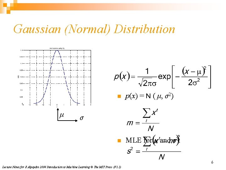
Gaussian (Normal) Distribution μ n p(x) = N ( μ, σ2) n MLE for μ and σ2: σ 6 Lecture Notes for E Alpaydın 2004 Introduction to Machine Learning © The MIT Press (V 1. 1)

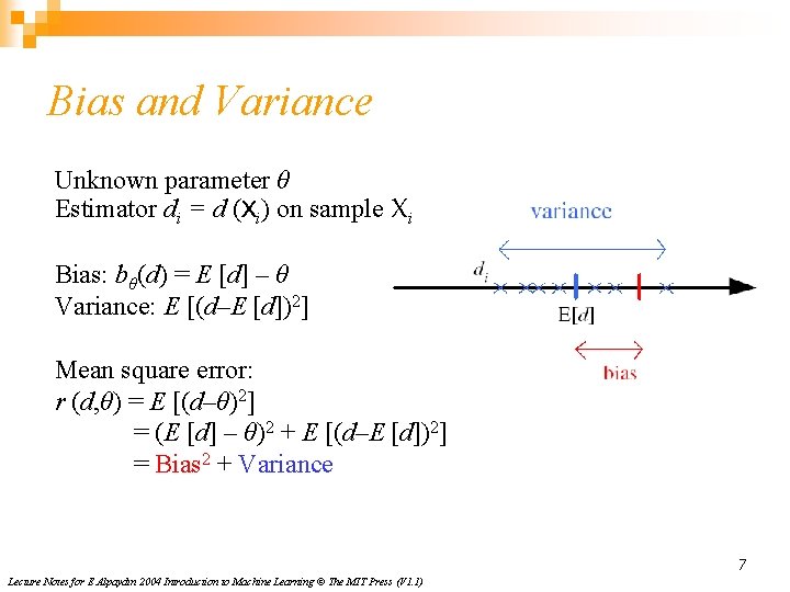
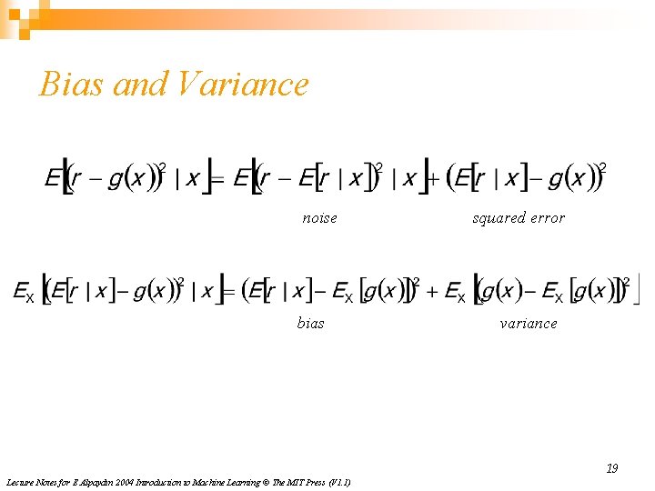
Bias and Variance Unknown parameter θ Estimator di = d (Xi) on sample Xi Bias: bθ(d) = E [d] – θ Variance: E [(d–E [d])2] Mean square error: r (d, θ) = E [(d–θ)2] = (E [d] – θ)2 + E [(d–E [d])2] = Bias 2 + Variance 7 Lecture Notes for E Alpaydın 2004 Introduction to Machine Learning © The MIT Press (V 1. 1)

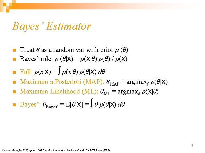
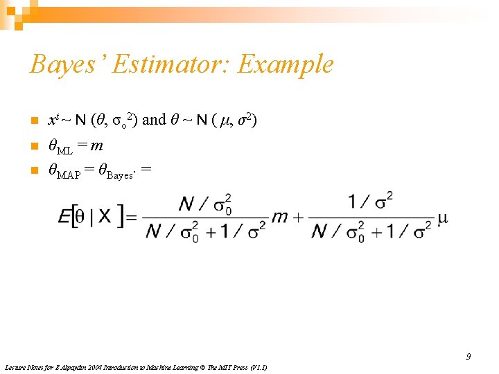
Bayes’ Estimator n n Treat θ as a random var with prior p (θ) Bayes’ rule: p (θ|X) = p(X|θ) p(θ) / p(X) n Full: p(x|X) = ∫ p(x|θ) p(θ|X) dθ Maximum a Posteriori (MAP): θMAP = argmaxθ p(θ|X) Maximum Likelihood (ML): θML = argmaxθ p(X|θ) n Bayes’: θBayes’ = E[θ|X] = ∫ θ p(θ|X) dθ n n 8 Lecture Notes for E Alpaydın 2004 Introduction to Machine Learning © The MIT Press (V 1. 1)

Bayes’ Estimator: Example n xt ~ N (θ, σo 2) and θ ~ N ( μ, σ2) n θML = m θMAP = θBayes’ = n 9 Lecture Notes for E Alpaydın 2004 Introduction to Machine Learning © The MIT Press (V 1. 1)

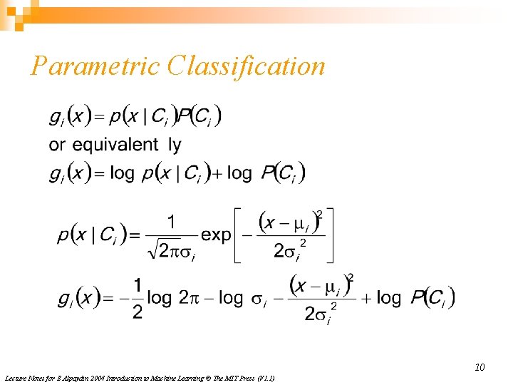
Parametric Classification 10 Lecture Notes for E Alpaydın 2004 Introduction to Machine Learning © The MIT Press (V 1. 1)

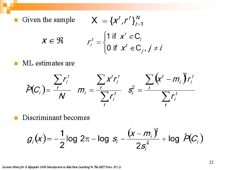
n Given the sample n ML estimates are n Discriminant becomes 11 Lecture Notes for E Alpaydın 2004 Introduction to Machine Learning © The MIT Press (V 1. 1)

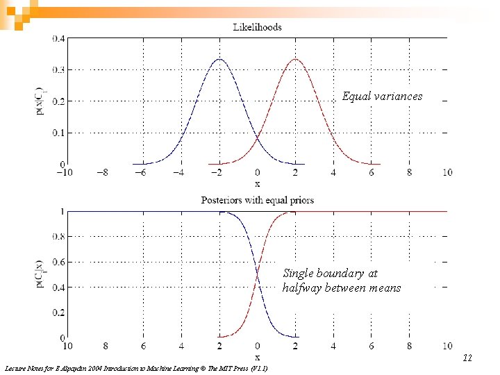
Equal variances Single boundary at halfway between means 12 Lecture Notes for E Alpaydın 2004 Introduction to Machine Learning © The MIT Press (V 1. 1)

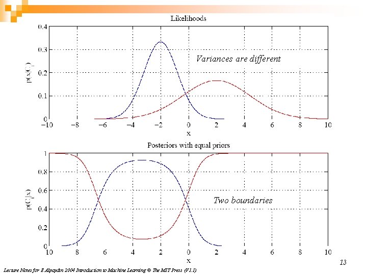
Variances are different Two boundaries 13 Lecture Notes for E Alpaydın 2004 Introduction to Machine Learning © The MIT Press (V 1. 1)

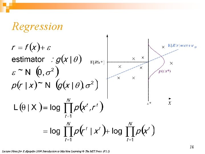
Regression 14 Lecture Notes for E Alpaydın 2004 Introduction to Machine Learning © The MIT Press (V 1. 1)

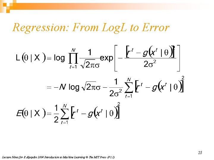
Regression: From Log. L to Error 15 Lecture Notes for E Alpaydın 2004 Introduction to Machine Learning © The MIT Press (V 1. 1)

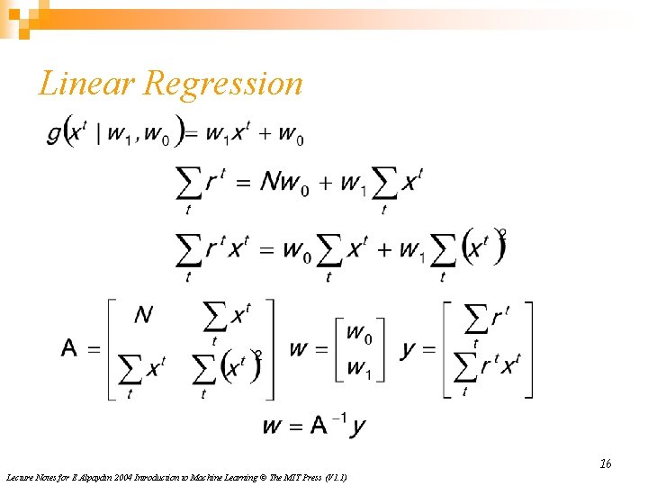
Linear Regression 16 Lecture Notes for E Alpaydın 2004 Introduction to Machine Learning © The MIT Press (V 1. 1)

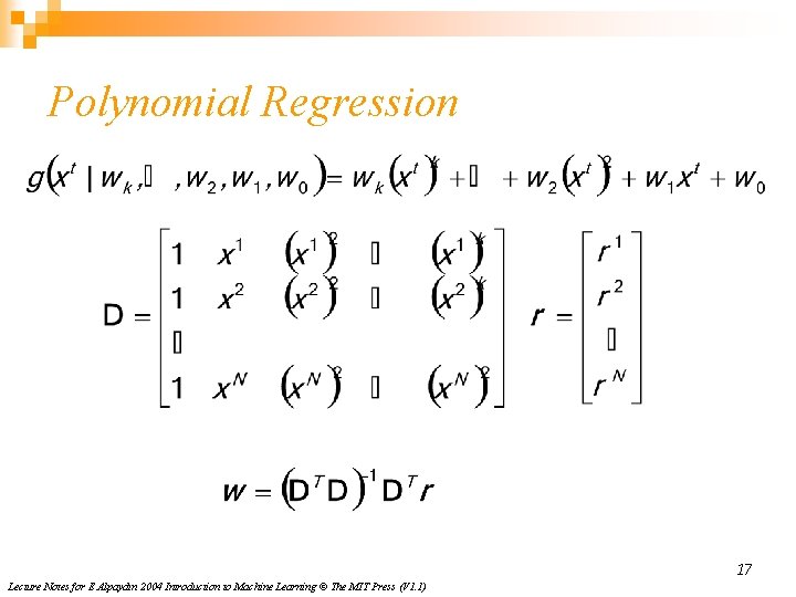
Polynomial Regression 17 Lecture Notes for E Alpaydın 2004 Introduction to Machine Learning © The MIT Press (V 1. 1)

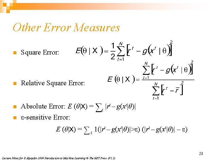
Other Error Measures n Square Error: n Relative Square Error: n Absolute Error: E (θ|X) = ∑t |rt – g(xt|θ)| n ε-sensitive Error: E (θ|X) = ∑ t 1(|rt – g(xt|θ)|>ε) (|rt – g(xt|θ)| – ε) 18 Lecture Notes for E Alpaydın 2004 Introduction to Machine Learning © The MIT Press (V 1. 1)

Bias and Variance noise bias squared error variance 19 Lecture Notes for E Alpaydın 2004 Introduction to Machine Learning © The MIT Press (V 1. 1)

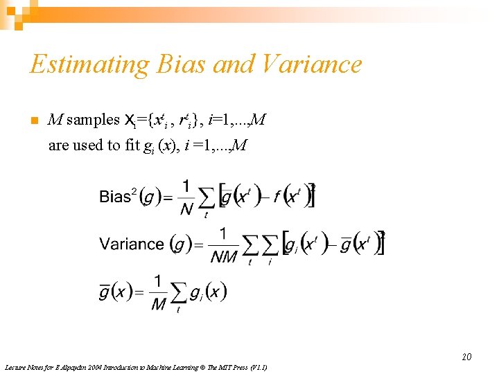
Estimating Bias and Variance n M samples Xi={xti , rti}, i=1, . . . , M are used to fit gi (x), i =1, . . . , M 20 Lecture Notes for E Alpaydın 2004 Introduction to Machine Learning © The MIT Press (V 1. 1)

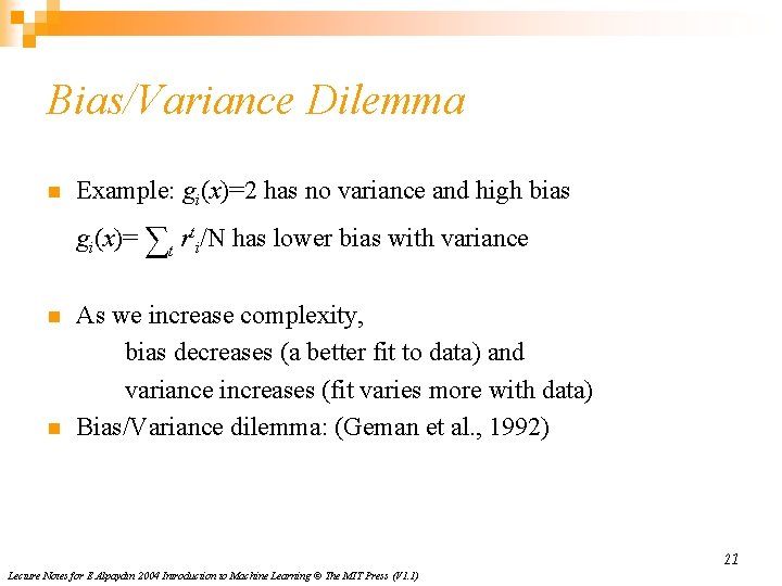
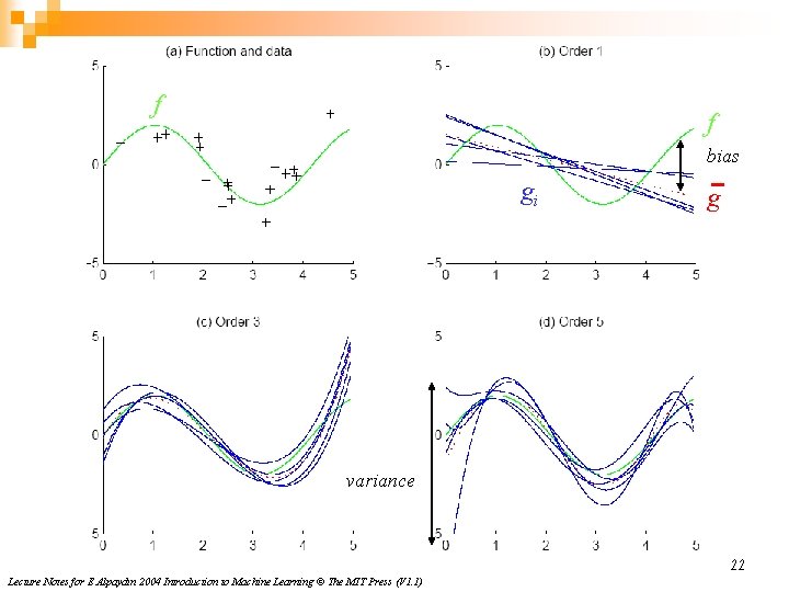
Bias/Variance Dilemma n Example: gi(x)=2 has no variance and high bias gi(x)= ∑t rti/N has lower bias with variance n n As we increase complexity, bias decreases (a better fit to data) and variance increases (fit varies more with data) Bias/Variance dilemma: (Geman et al. , 1992) 21 Lecture Notes for E Alpaydın 2004 Introduction to Machine Learning © The MIT Press (V 1. 1)

f f bias gi g variance 22 Lecture Notes for E Alpaydın 2004 Introduction to Machine Learning © The MIT Press (V 1. 1)

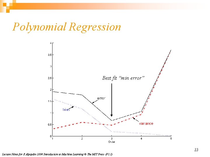
Polynomial Regression Best fit “min error” 23 Lecture Notes for E Alpaydın 2004 Introduction to Machine Learning © The MIT Press (V 1. 1)

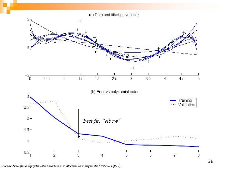
Best fit, “elbow” 24 Lecture Notes for E Alpaydın 2004 Introduction to Machine Learning © The MIT Press (V 1. 1)

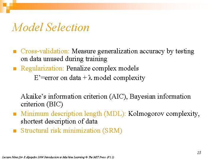
Model Selection n n Cross-validation: Measure generalization accuracy by testing on data unused during training Regularization: Penalize complex models E’=error on data + λ model complexity Akaike’s information criterion (AIC), Bayesian information criterion (BIC) Minimum description length (MDL): Kolmogorov complexity, shortest description of data Structural risk minimization (SRM) 25 Lecture Notes for E Alpaydın 2004 Introduction to Machine Learning © The MIT Press (V 1. 1)

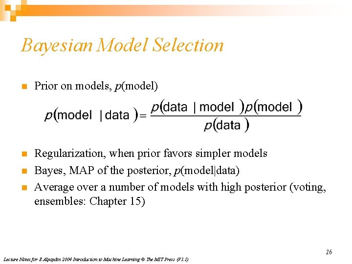
Bayesian Model Selection n Prior on models, p(model) n Regularization, when prior favors simpler models Bayes, MAP of the posterior, p(model|data) Average over a number of models with high posterior (voting, ensembles: Chapter 15) n n 26 Lecture Notes for E Alpaydın 2004 Introduction to Machine Learning © The MIT Press (V 1. 1)