Lecture Slides for INTRODUCTION TO MACHINE LEARNING 3

Lecture Slides for INTRODUCTION TO MACHINE LEARNING 3 RD EDITION ETHEM ALPAYDIN © The MIT Press, 2014 Modified by Prof. Carolina Ruiz for CS 539 Machine Learning at WPI alpaydin@boun. edu. tr http: //www. cmpe. boun. edu. tr/~ethem/i 2 ml 3 e

CHAPTER 6: DIMENSIONALITY REDUCTION

Why Reduce Dimensionality? 3 Reduces time complexity: Less computation Reduces space complexity: Fewer parameters Saves the cost of observing the feature Simpler models are more robust on small datasets More interpretable; simpler explanation Data visualization (structure, groups, outliers, etc) if plotted in 2 or 3 dimensions

Feature Selection vs Extraction 4 Feature selection: Choosing k<d important features, ignoring the remaining d – k Subset selection algorithms Feature extraction: Project the original xi , i =1, . . . , d dimensions to new k<d dimensions, zj , j =1, . . . , k

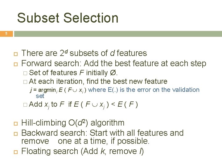
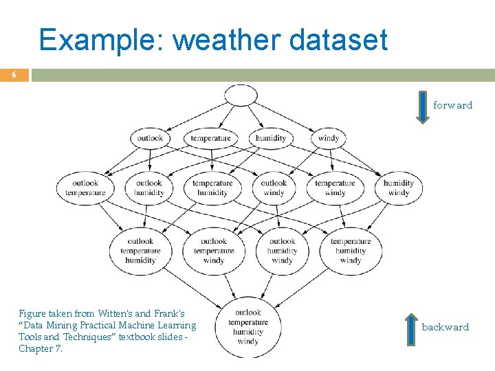
Subset Selection 5 There are 2 d subsets of d features Forward search: Add the best feature at each step � Set of features F initially Ø. � At each iteration, find the best new feature j = argmini E ( F È xi ) where E(. ) is the error on the validation set � Add xj to F if E ( F È xj ) < E ( F ) Hill-climbing O(d 2) algorithm Backward search: Start with all features and remove one at a time, if possible. Floating search (Add k, remove l)

Example: weather dataset 6 forward Figure taken from Witten's and Frank's “Data Mining Practical Machine Learning Tools and Techniques” textbook slides Chapter 7. backward

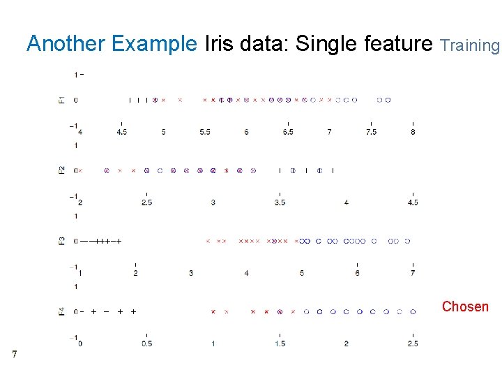
Another Example Iris data: Single feature Training Chosen 7

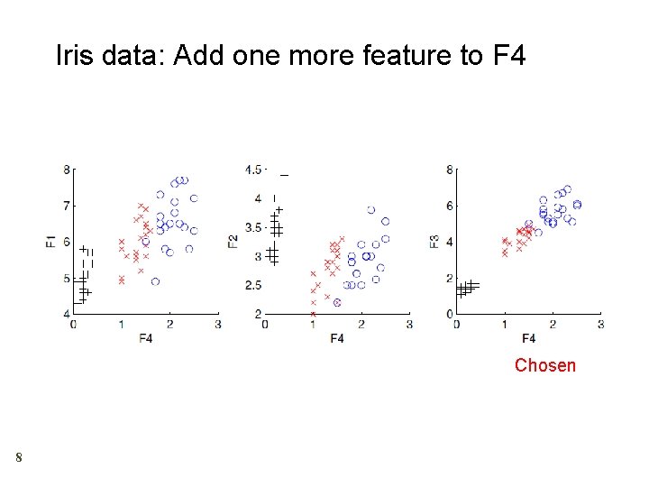
Iris data: Add one more feature to F 4 Chosen 8

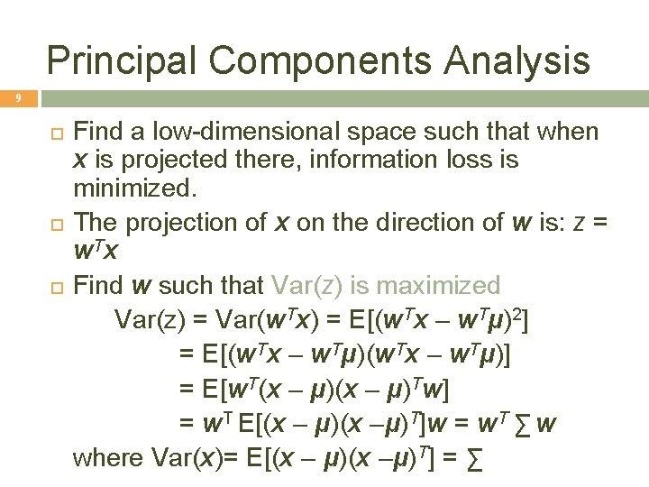
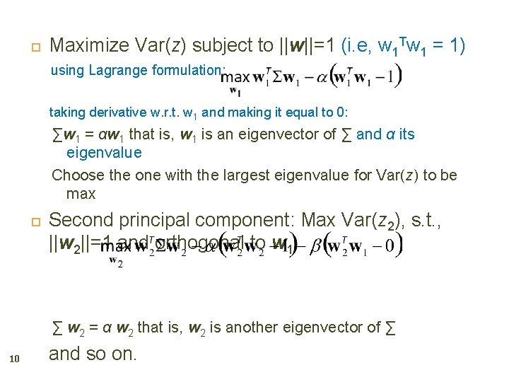
Principal Components Analysis 9 Find a low-dimensional space such that when x is projected there, information loss is minimized. The projection of x on the direction of w is: z = w Tx Find w such that Var(z) is maximized Var(z) = Var(w. Tx) = E[(w. Tx – w. Tμ)2] = E[(w. Tx – w. Tμ)] = E[w. T(x – μ)Tw] = w. T E[(x – μ)(x –μ)T]w = w. T ∑ w where Var(x)= E[(x – μ)(x –μ)T] = ∑

Maximize Var(z) subject to ||w||=1 (i. e, w 1 Tw 1 = 1) using Lagrange formulation: taking derivative w. r. t. w 1 and making it equal to 0: ∑w 1 = αw 1 that is, w 1 is an eigenvector of ∑ and α its eigenvalue Choose the one with the largest eigenvalue for Var(z) to be max Second principal component: Max Var(z 2), s. t. , ||w 2||=1 and orthogonal to w 1 ∑ w 2 = α w 2 that is, w 2 is another eigenvector of ∑ 10 and so on.

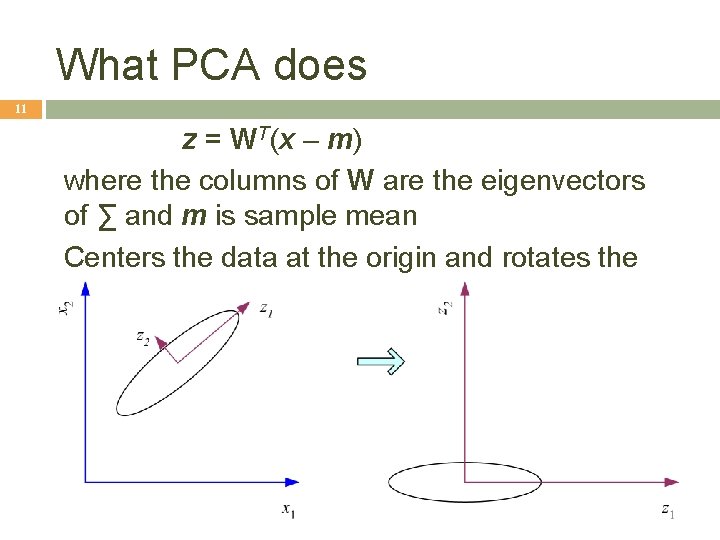
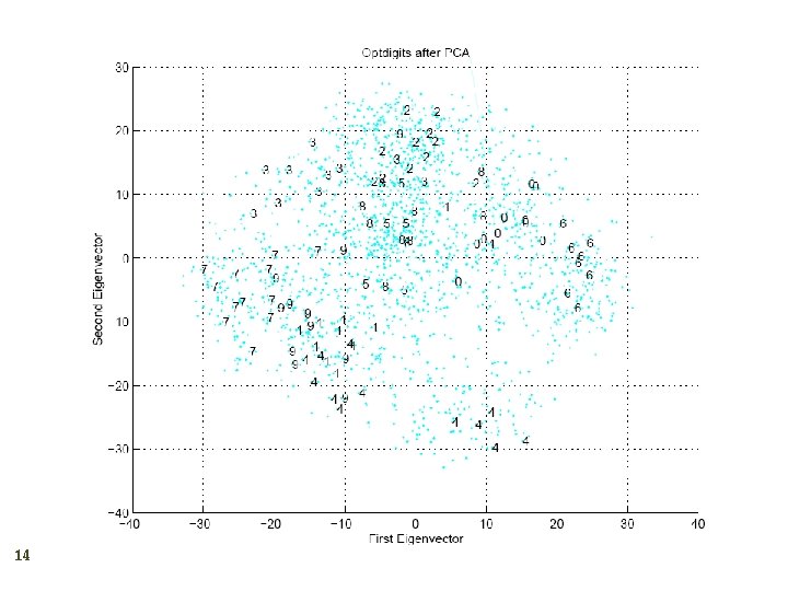
What PCA does 11 z = WT(x – m) where the columns of W are the eigenvectors of ∑ and m is sample mean Centers the data at the origin and rotates the axes

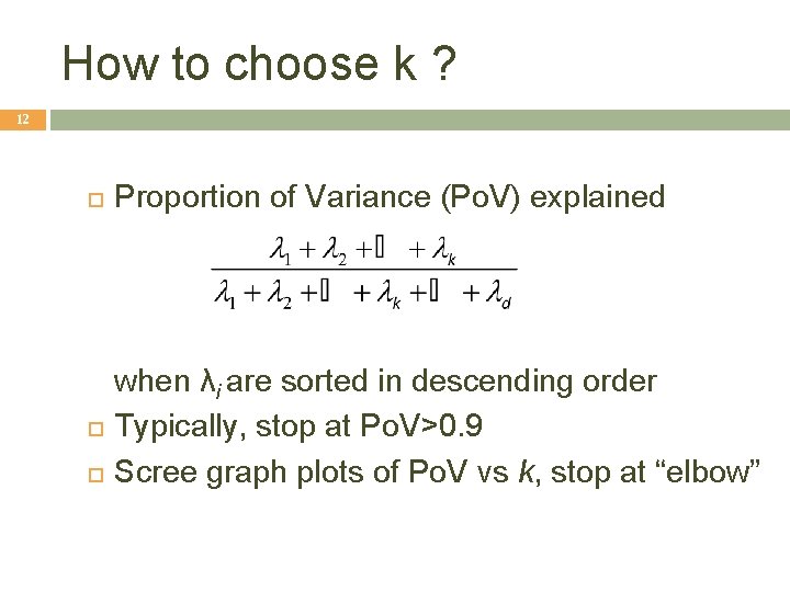
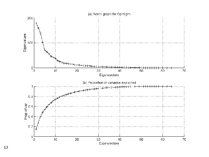
How to choose k ? 12 Proportion of Variance (Po. V) explained when λi are sorted in descending order Typically, stop at Po. V>0. 9 Scree graph plots of Po. V vs k, stop at “elbow”

13

14

Feature Embedding 15 When X is the Nxd data matrix, XTX is the dxd matrix (covariance of features, if meancentered) XXT is the Nx. N matrix (pairwise similarities of instances) PCA uses the eigenvectors of XTX which are d-dim and can be used for projection Feature embedding uses the eigenvectors of XXT which are N-dim and which give directly the coordinates after projection Sometimes, we can define pairwise similarities (or distances) between instances, then we can use feature embedding without needing to represent instances as vectors.

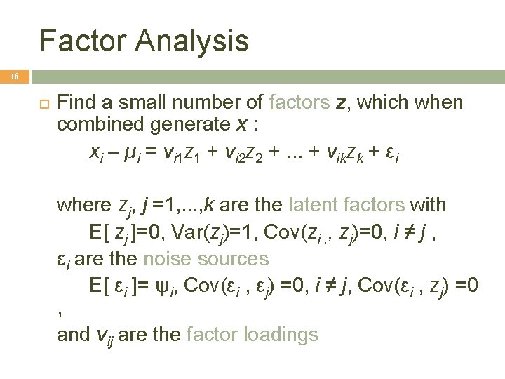
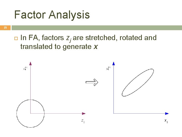
Factor Analysis 16 Find a small number of factors z, which when combined generate x : xi – µi = vi 1 z 1 + vi 2 z 2 +. . . + vikzk + εi where zj, j =1, . . . , k are the latent factors with E[ zj ]=0, Var(zj)=1, Cov(zi , , zj)=0, i ≠ j , εi are the noise sources E[ εi ]= ψi, Cov(εi , εj) =0, i ≠ j, Cov(εi , zj) =0 , and vij are the factor loadings

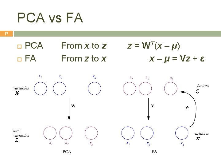
PCA vs FA 17 PCA FA From x to z From z to x z = WT(x – µ) x – µ = Vz + ε x z z x

Factor Analysis 18 In FA, factors zj are stretched, rotated and translated to generate x

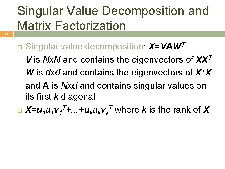
19 Singular Value Decomposition and Matrix Factorization Singular value decomposition: X=VAWT V is Nx. N and contains the eigenvectors of XXT W is dxd and contains the eigenvectors of XTX and A is Nxd and contains singular values on its first k diagonal X=u 1 a 1 v 1 T+. . . +ukakvk. T where k is the rank of X

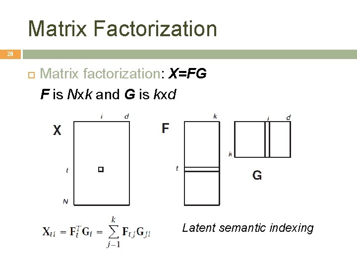
Matrix Factorization 20 Matrix factorization: X=FG F is Nxk and G is kxd Latent semantic indexing

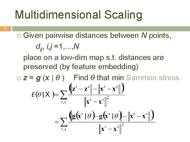
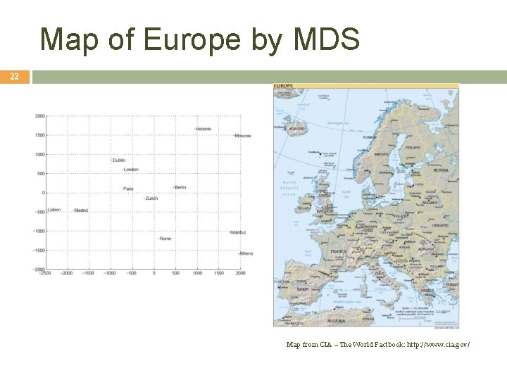
Multidimensional Scaling 21 Given pairwise distances between N points, dij, i, j =1, . . . , N place on a low-dim map s. t. distances are preserved (by feature embedding) z = g (x | θ ) Find θ that min Sammon stress

Map of Europe by MDS 22 Map from CIA – The World Factbook: http: //www. cia. gov/

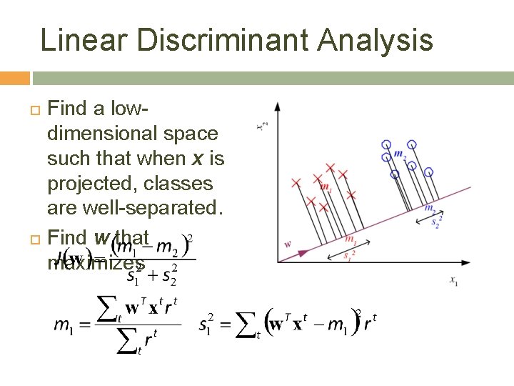
Linear Discriminant Analysis Find a lowdimensional space such that when x is projected, classes are well-separated. Find w that maximizes 23

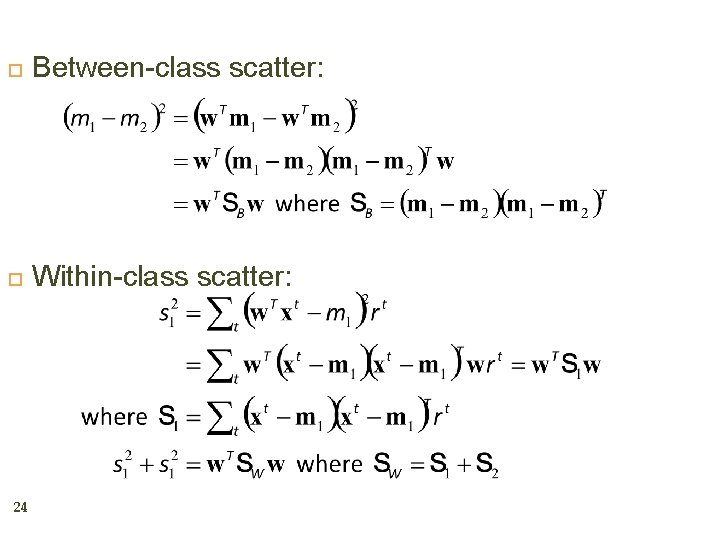
Between-class scatter: Within-class scatter: 24

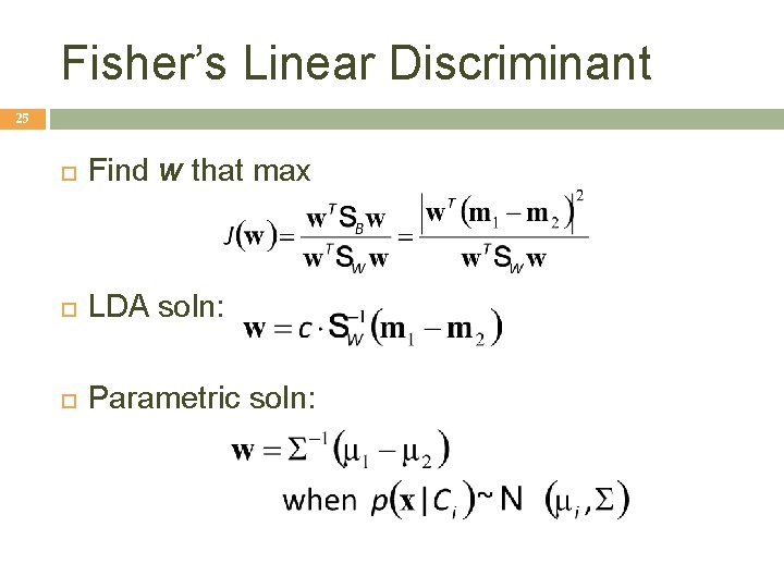
Fisher’s Linear Discriminant 25 Find w that max LDA soln: Parametric soln:

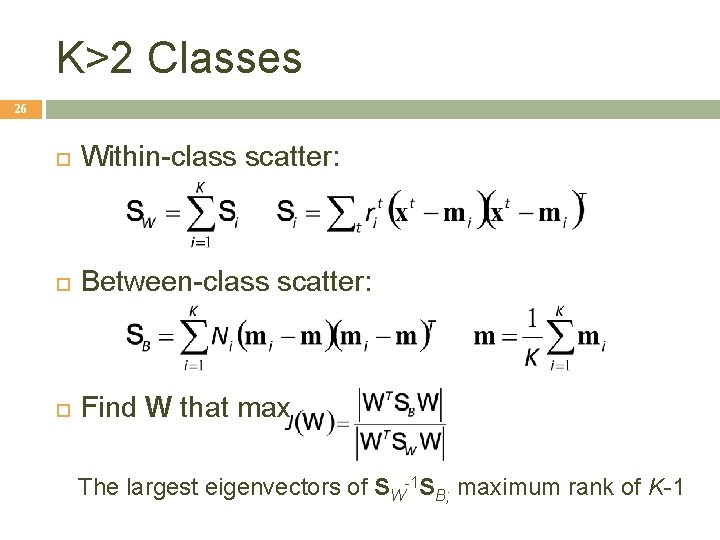
K>2 Classes 26 Within-class scatter: Between-class scatter: Find W that max The largest eigenvectors of SW-1 SB; maximum rank of K-1

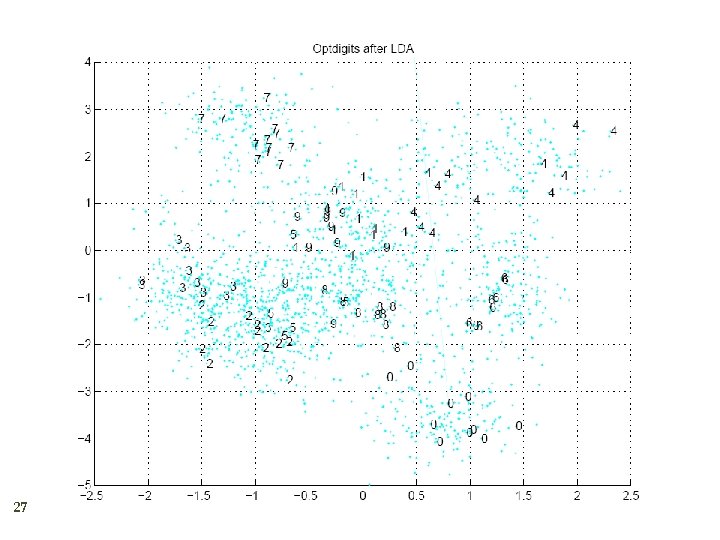
27

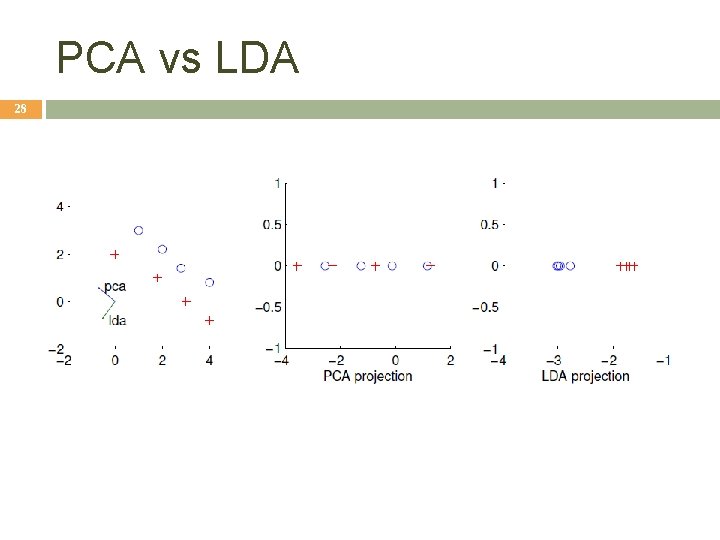
PCA vs LDA 28

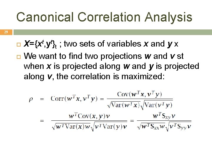
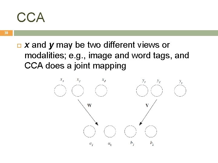
Canonical Correlation Analysis 29 X={xt, yt}t ; two sets of variables x and y x We want to find two projections w and v st when x is projected along w and y is projected along v, the correlation is maximized:

CCA 30 x and y may be two different views or modalities; e. g. , image and word tags, and CCA does a joint mapping

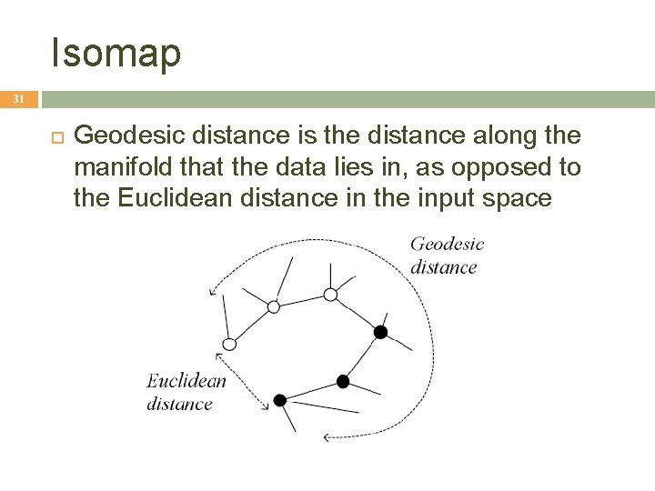
Isomap 31 Geodesic distance is the distance along the manifold that the data lies in, as opposed to the Euclidean distance in the input space

Isomap 32 Instances r and s are connected in the graph if ||xr-xs||<e or if xs is one of the k neighbors of xr The edge length is ||xr-xs|| For two nodes r and s not connected, the distance is equal to the shortest path between them Once the Nx. N distance matrix is thus formed, use MDS to find a lower-dimensional mapping

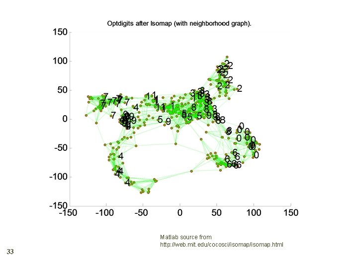
33 Matlab source from http: //web. mit. edu/cocosci/isomap. html

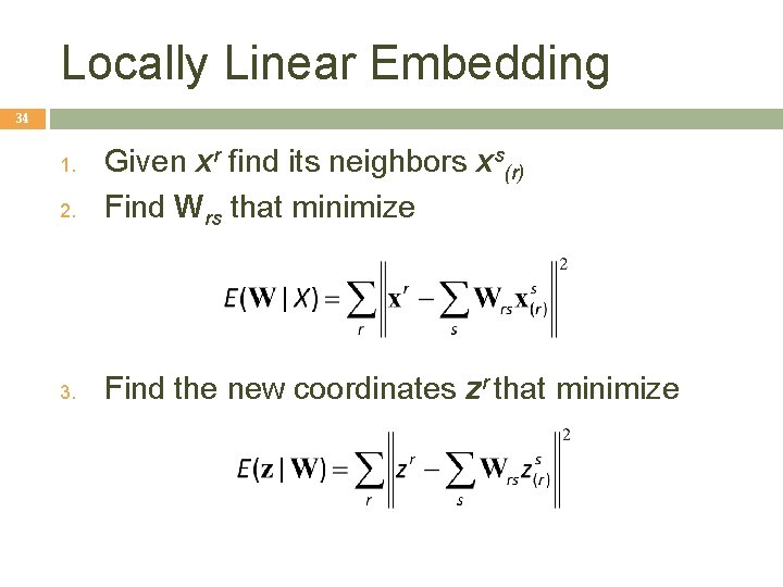
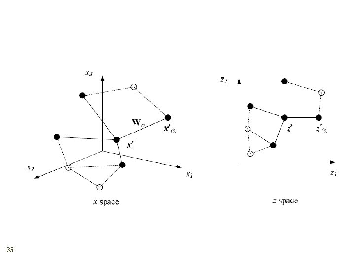
Locally Linear Embedding 34 2. Given xr find its neighbors xs(r) Find Wrs that minimize 3. Find the new coordinates zr that minimize 1.

35

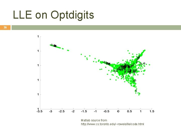
LLE on Optdigits 36 Matlab source from http: //www. cs. toronto. edu/~roweis/lle/code. html

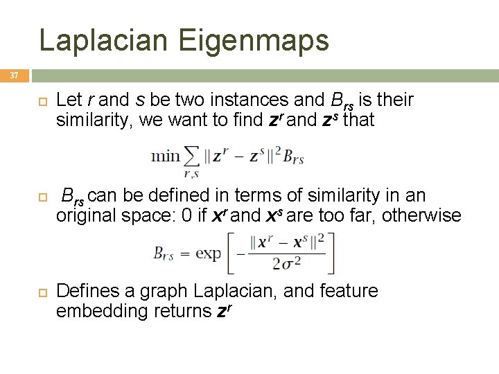
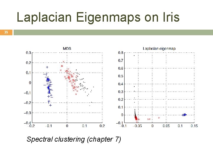
Laplacian Eigenmaps 37 Let r and s be two instances and Brs is their similarity, we want to find zr and zs that Brs can be defined in terms of similarity in an original space: 0 if xr and xs are too far, otherwise Defines a graph Laplacian, and feature embedding returns zr

Laplacian Eigenmaps on Iris 38 Spectral clustering (chapter 7)