Lecture Slides for INTRODUCTION TO MACHINE LEARNING 3

Lecture Slides for INTRODUCTION TO MACHINE LEARNING 3 RD EDITION ETHEM ALPAYDIN © The MIT Press, 2014 at WPI Modified by Prof. Carolina Ruiz for CS 539 Machine Learning alpaydin@boun. edu. tr http: //www. cmpe. boun. edu. tr/~ethem/i 2 ml 3 e

CHAPTER 4: PARAMETRIC METHODS

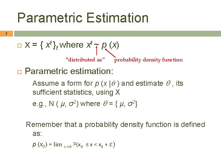
Parametric Estimation 3 X = { xt }t where xt ~ p (x) “distributed as” probability density function Parametric estimation: Assume a form for p (x |q ) and estimate q , its sufficient statistics, using X e. g. , N ( μ, σ2) where q = { μ, σ2} Remember that a probability density function is defined as: p (x 0) ≡ lim ε→ 0 P(x 0 ≤ x < x 0 + ε)

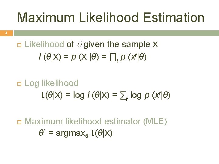
Maximum Likelihood Estimation 4 Likelihood of q given the sample X l (θ|X) = p (X |θ) = ∏t p (xt|θ) Log likelihood L(θ|X) = log l (θ|X) = ∑t log p (xt|θ) Maximum likelihood estimator (MLE) θ* = argmaxθ L(θ|X)

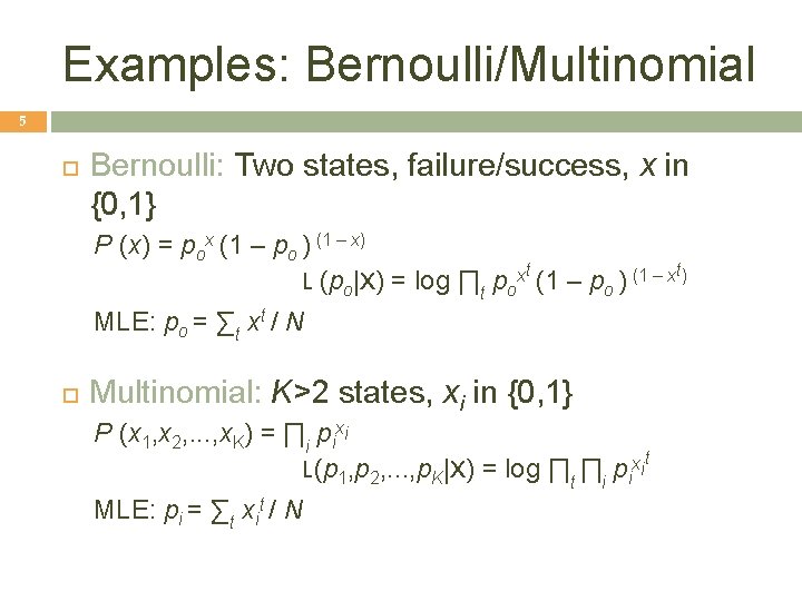
Examples: Bernoulli/Multinomial 5 Bernoulli: Two states, failure/success, x in {0, 1} P (x) = pox (1 – po ) (1 – x) L (po|X) = log ∏t poxt (1 – po ) (1 – xt) MLE: po = ∑t xt / N Multinomial: K>2 states, xi in {0, 1} P (x 1, x 2, . . . , x. K) = ∏i pixi L(p 1, p 2, . . . , p. K|X) = log ∏t ∏i pixit MLE: pi = ∑t xit / N

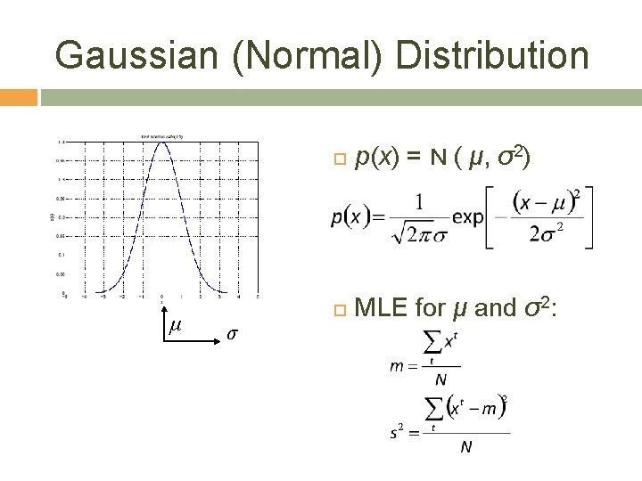
Gaussian (Normal) Distribution μ σ p(x) = N ( μ, σ2) MLE for μ and σ2: 6

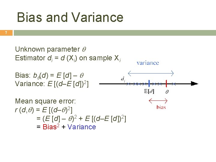
Bias and Variance 7 Unknown parameter q Estimator di = d (Xi) on sample Xi Bias: bq(d) = E [d] – q Variance: E [(d–E [d])2] q Mean square error: r (d, q) = E [(d–q)2] = (E [d] – q)2 + E [(d–E [d])2] = Bias 2 + Variance

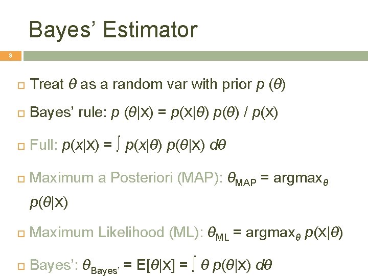
Bayes’ Estimator 8 Treat θ as a random var with prior p (θ) Bayes’ rule: p (θ|X) = p(X|θ) p(θ) / p(X) Full: p(x|X) = ∫ p(x|θ) p(θ|X) dθ Maximum a Posteriori (MAP): θMAP = argmaxθ p(θ|X) Maximum Likelihood (ML): θML = argmaxθ p(X|θ) Bayes’: θBayes’ = E[θ|X] = ∫ θ p(θ|X) dθ

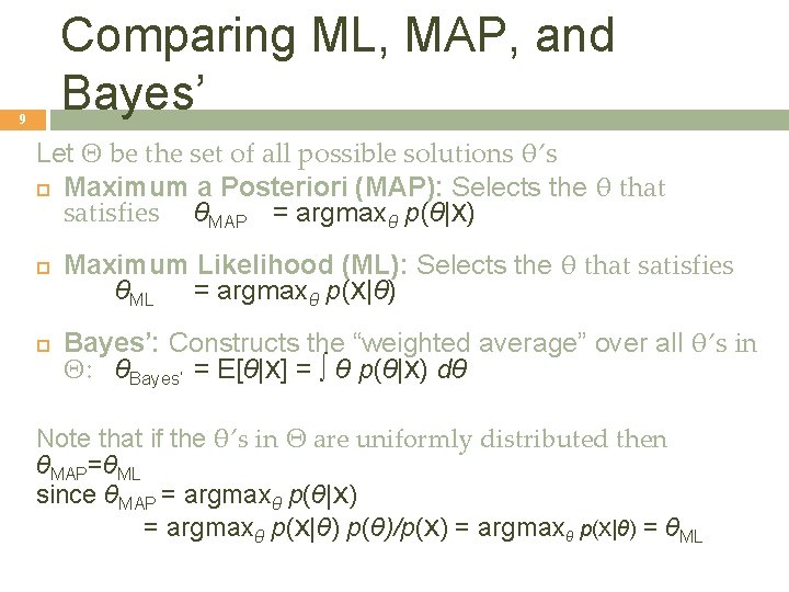
Comparing ML, MAP, and Bayes’ 9 Let Θ be the set of all possible solutions θ’s Maximum a Posteriori (MAP): Selects the θ that satisfies θMAP = argmaxθ p(θ|X) Maximum Likelihood (ML): Selects the θ that satisfies θML = argmaxθ p(X|θ) Bayes’: Constructs the “weighted average” over all θ’s in Θ: θBayes’ = E[θ|X] = ∫ θ p(θ|X) dθ Note that if the θ’s in Θ are uniformly distributed then θMAP=θML since θMAP = argmaxθ p(θ|X) = argmaxθ p(X|θ) p(θ)/p(X) = argmaxθ p(X|θ) = θML

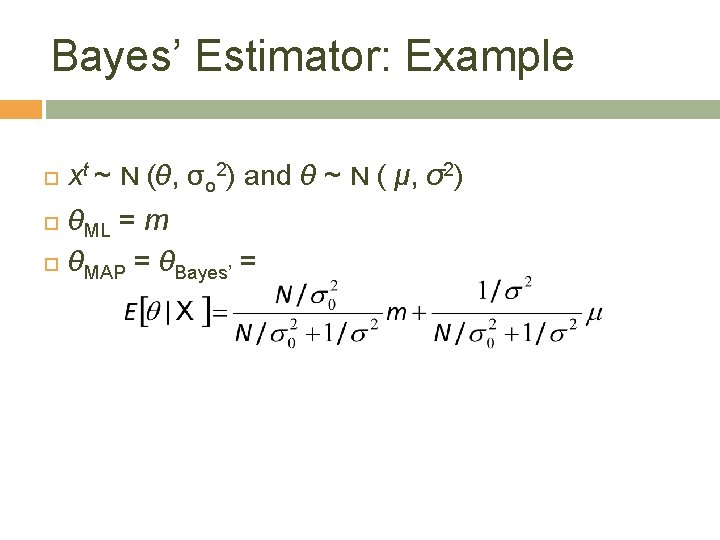
Bayes’ Estimator: Example xt ~ N (θ, σo 2) and θ ~ N ( μ, σ2) θML = m θMAP = θBayes’ = 10

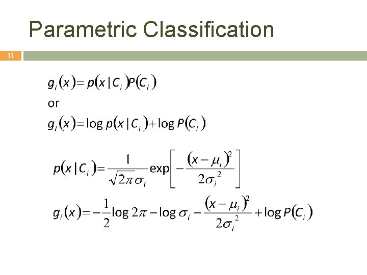
Parametric Classification 11

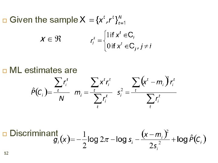
Given the sample ML estimates are Discriminant 12

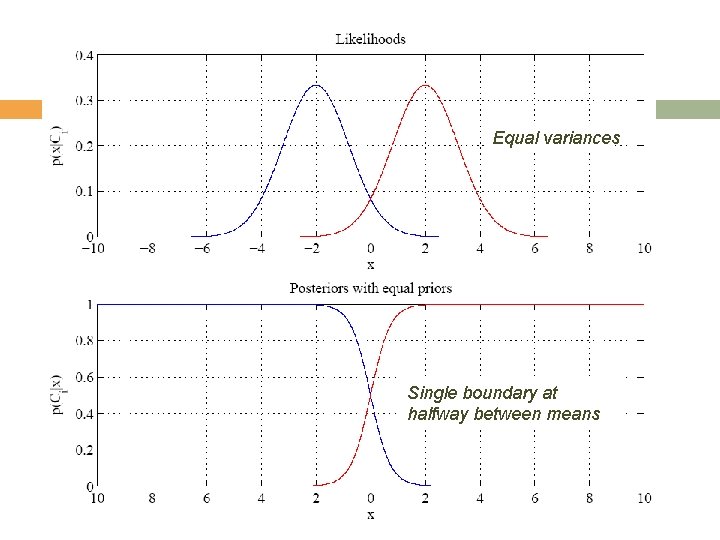
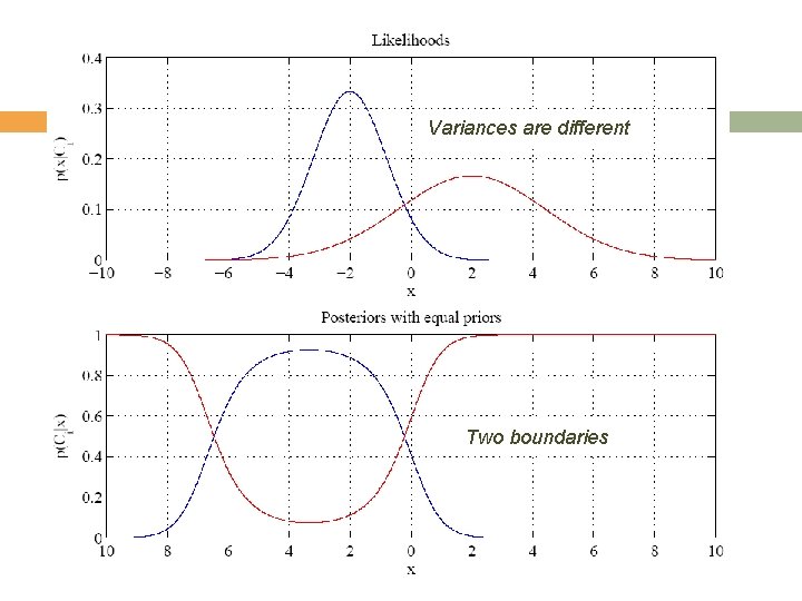
Equal variances Single boundary at halfway between means 13

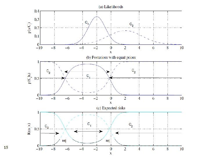
Variances are different Two boundaries 14

15

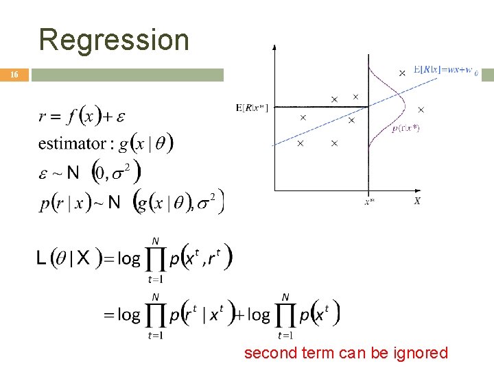
Regression 16 second term can be ignored

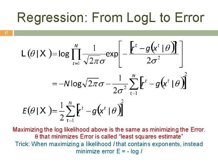
Regression: From Log. L to Error 17 Maximizing the log likelihood above is the same as minimizing the Error. θ that minimizes Error is called “least squares estimate” Trick: When maximizing a likelihood l that contains exponents, instead minimize error E = - log l

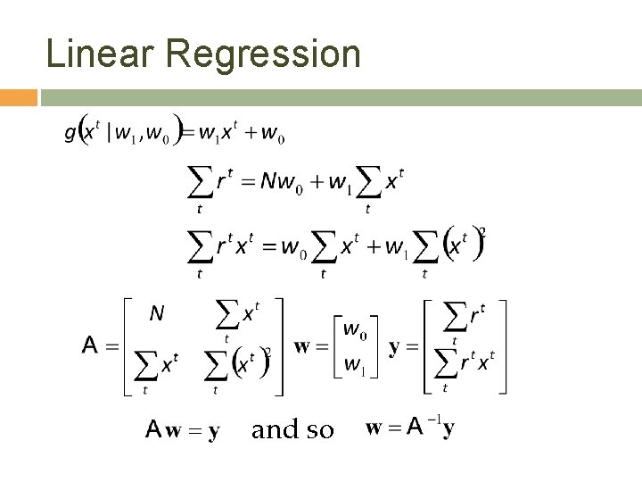
Linear Regression and so 18

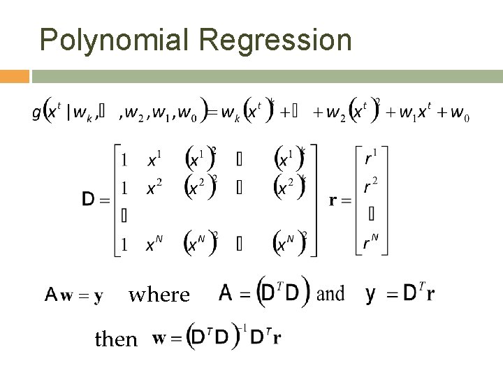
Polynomial Regression where then 19

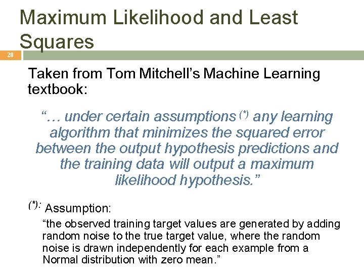
20 Maximum Likelihood and Least Squares Taken from Tom Mitchell’s Machine Learning textbook: “… under certain assumptions (*) any learning algorithm that minimizes the squared error between the output hypothesis predictions and the training data will output a maximum likelihood hypothesis. ” (*): Assumption: “the observed training target values are generated by adding random noise to the true target value, where the random noise is drawn independently for each example from a Normal distribution with zero mean. ”

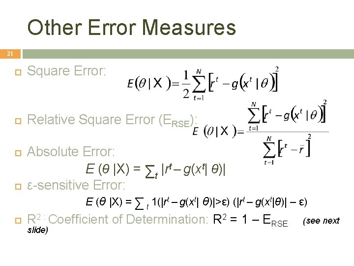
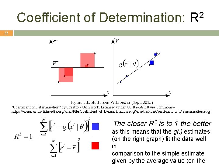
Other Error Measures 21 Square Error: Relative Square Error (ERSE): Absolute Error: E (θ |X) = ∑t |rt – g(xt| θ)| ε-sensitive Error: E (θ |X) = ∑ t 1(|rt – g(xt| θ)|>ε) (|rt – g(xt|θ)| – ε) R 2 : Coefficient of Determination: R 2 = 1 – ERSE (see next slide)

Coefficient of Determination: R 2 22 Figure adapted from Wikipedia (Sept. 2015) "Coefficient of Determination" by Orzetto - Own work. Licensed under CC BY-SA 3. 0 via Commons – https: //commons. wikimedia. org/wiki/File: Coefficient_of_Determination. svg#/media/File: Coefficient_of_Determination. svg The closer R 2 is to 1 the better as this means that the g(. ) estimates (on the right graph) fit the data well in comparison to the simple estimate given by the average value (on the

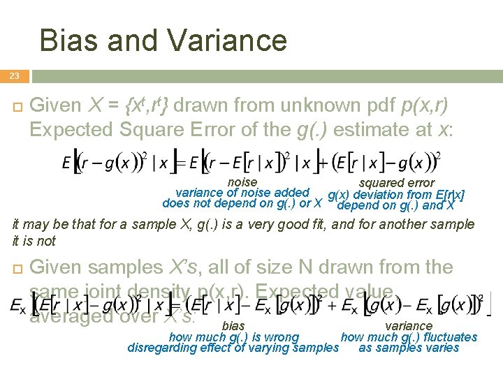
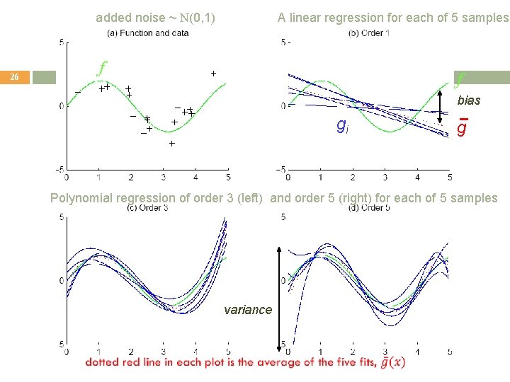
Bias and Variance 23 Given X = {xt, rt} drawn from unknown pdf p(x, r) Expected Square Error of the g(. ) estimate at x: noise squared error variance of noise added g(x) deviation from E[r|x] does not depend on g(. ) or X depend on g(. ) and X it may be that for a sample X, g(. ) is a very good fit, and for another sample it is not Given samples X’s, all of size N drawn from the same joint density p(x, r). Expected value, averaged over X’s: bias variance how much g(. ) is wrong how much g(. ) fluctuates disregarding effect of varying samples as samples varies

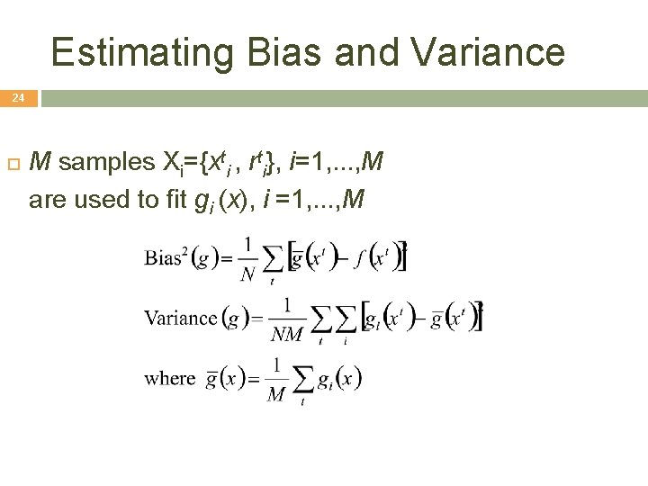
Estimating Bias and Variance 24 M samples Xi={xti , rti}, i=1, . . . , M are used to fit gi (x), i =1, . . . , M

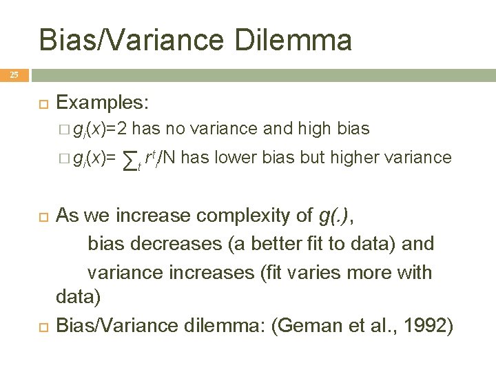
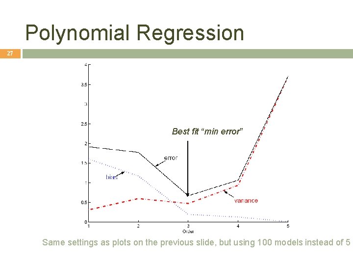
Bias/Variance Dilemma 25 Examples: � gi(x)=2 � gi(x)= has no variance and high bias ∑t rti/N has lower bias but higher variance As we increase complexity of g(. ), bias decreases (a better fit to data) and variance increases (fit varies more with data) Bias/Variance dilemma: (Geman et al. , 1992)

added noise ~ N(0, 1) A linear regression for each of 5 samples f 26 f bias gi g Polynomial regression of order 3 (left) and order 5 (right) for each of 5 samples variance

Polynomial Regression 27 Best fit “min error” Same settings as plots on the previous slide, but using 100 models instead of 5

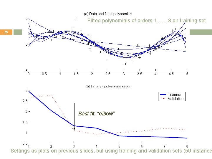
Fitted polynomials of orders 1, …, 8 on training set 28 Best fit, “elbow” Settings as plots on previous slides, but using training and validation sets (50 instance

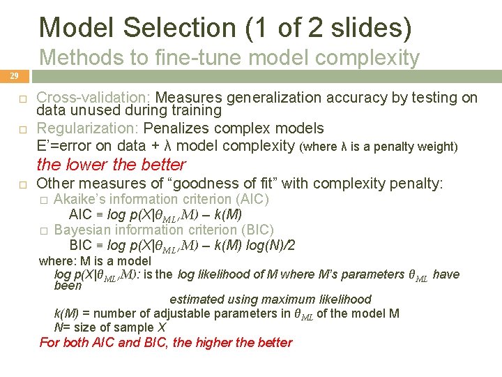
Model Selection (1 of 2 slides) Methods to fine-tune model complexity 29 Cross-validation: Measures generalization accuracy by testing on data unused during training Regularization: Penalizes complex models E’=error on data + λ model complexity (where λ is a penalty weight) the lower the better Other measures of “goodness of fit” with complexity penalty: � � Akaike’s information criterion (AIC) AIC ≡ log p(X|θML, M) – k(M) Bayesian information criterion (BIC) BIC ≡ log p(X|θML, M) – k(M) log(N)/2 where: M is a model log p(X|θML, M): is the log likelihood of M where M’s parameters θML have been estimated using maximum likelihood k(M) = number of adjustable parameters in θML of the model M N= size of sample X For both AIC and BIC, the higher the better

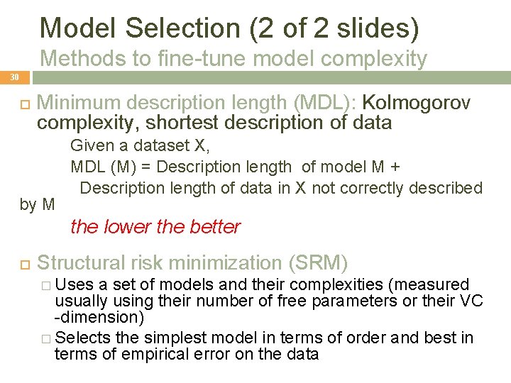
Model Selection (2 of 2 slides) Methods to fine-tune model complexity 30 Minimum description length (MDL): Kolmogorov complexity, shortest description of data by M Given a dataset X, MDL (M) = Description length of model M + Description length of data in X not correctly described the lower the better Structural risk minimization (SRM) � Uses a set of models and their complexities (measured usually using their number of free parameters or their VC -dimension) � Selects the simplest model in terms of order and best in terms of empirical error on the data

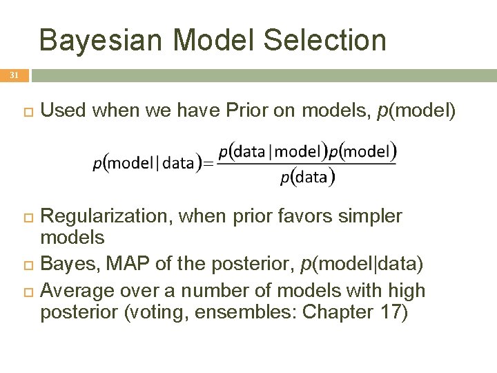
Bayesian Model Selection 31 Used when we have Prior on models, p(model) Regularization, when prior favors simpler models Bayes, MAP of the posterior, p(model|data) Average over a number of models with high posterior (voting, ensembles: Chapter 17)

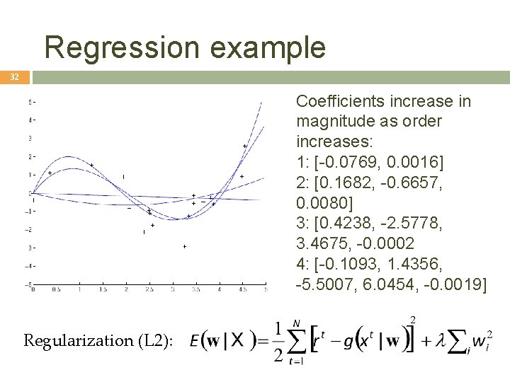
Regression example 32 Coefficients increase in magnitude as order increases: 1: [-0. 0769, 0. 0016] 2: [0. 1682, -0. 6657, 0. 0080] 3: [0. 4238, -2. 5778, 3. 4675, -0. 0002 4: [-0. 1093, 1. 4356, -5. 5007, 6. 0454, -0. 0019] Regularization (L 2):