Lecture Slides for INTRODUCTION TO Machine Learning 2

Lecture Slides for INTRODUCTION TO Machine Learning 2 nd Edition ETHEM ALPAYDIN © The MIT Press, 2010 alpaydin@boun. edu. tr http: //www. cmpe. boun. edu. tr/~ethem/i 2 ml 2 e Lecture Notes for E Alpaydın 2010 Introduction to Machine Learning 2 e © The MIT Press (V 1. 0)

CHAPTER 6: Dimensionality Reduction Lecture Notes for E Alpaydın 2010 Introduction to Machine Learning 2 e © The MIT Press (V 1. 0)

Why Reduce Dimensionality? 1. 2. 3. 4. 5. 6. Reduces time complexity: Less computation Reduces space complexity: Less parameters Saves the cost of observing the features Simpler models are more robust on small datasets More interpretable; simpler explanation Data visualization (structure, groups, outliers, etc) if plotted in 2 or 3 dimensions Lecture Notes for E Alpaydın 2010 Introduction to Machine Learning 2 e © The MIT Press (V 1. 0) 3

Feature Selection vs Extraction �Feature selection: �Choosing k<d important features, ignoring the remaining d – k Subset selection algorithms � Rough Sets � �Feature extraction: �Project the original xi , i =1, . . . , d dimensions to new k<d dimensions, zj , j =1, . . . , k Principal components analysis (PCA) � Linear discriminant analysis (LDA) � Factor analysis (FA) Lecture Notes for E Alpaydın 2010 Introduction to Machine Learning 2 e © The MIT Press (V 1. 0) � 4

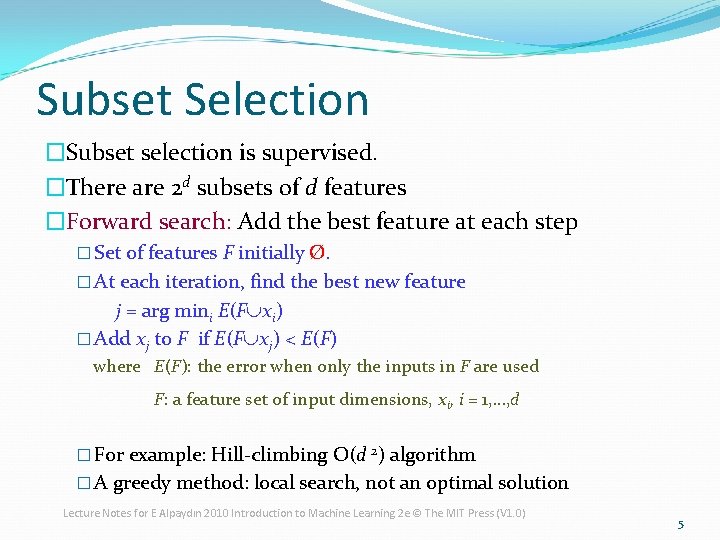
Subset Selection �Subset selection is supervised. �There are 2 d subsets of d features �Forward search: Add the best feature at each step � Set of features F initially Ø. � At each iteration, find the best new feature j = arg mini E(FÈxi) � Add xj to F if E(FÈxj) < E(F) where E(F): the error when only the inputs in F are used F: a feature set of input dimensions, xi, i = 1, …, d � For example: Hill-climbing O(d 2) algorithm � A greedy method: local search, not an optimal solution Lecture Notes for E Alpaydın 2010 Introduction to Machine Learning 2 e © The MIT Press (V 1. 0) 5

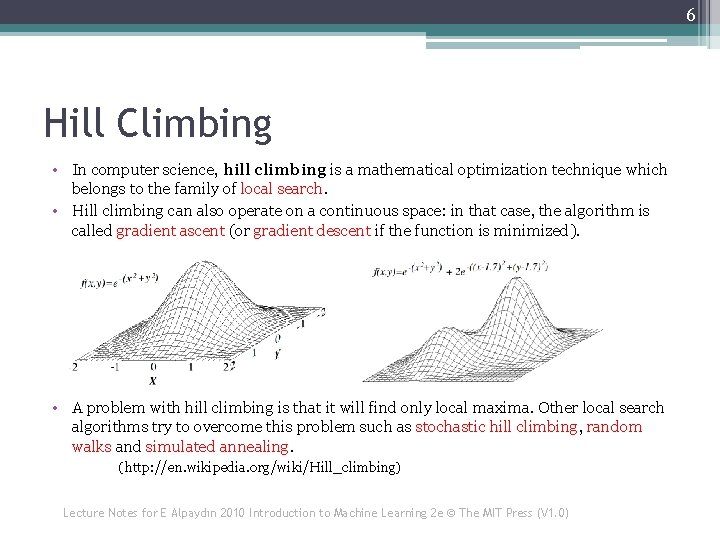
6 Hill Climbing • In computer science, hill climbing is a mathematical optimization technique which belongs to the family of local search. • Hill climbing can also operate on a continuous space: in that case, the algorithm is called gradient ascent (or gradient descent if the function is minimized). • A problem with hill climbing is that it will find only local maxima. Other local search algorithms try to overcome this problem such as stochastic hill climbing, random walks and simulated annealing. (http: //en. wikipedia. org/wiki/Hill_climbing) Lecture Notes for E Alpaydın 2010 Introduction to Machine Learning 2 e © The MIT Press (V 1. 0)

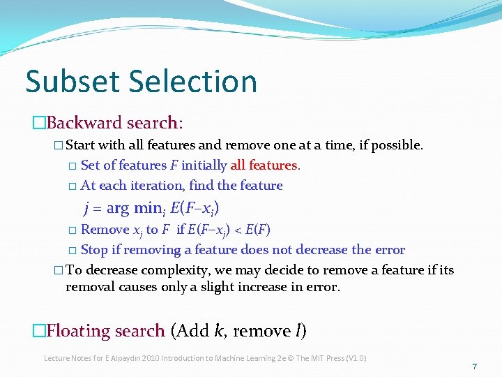
Subset Selection �Backward search: � Start with all features and remove one at a time, if possible. Set of features F initially all features. � At each iteration, find the feature � j = arg mini E(F-xi) Remove xj to F if E(F-xj) < E(F) � Stop if removing a feature does not decrease the error � To decrease complexity, we may decide to remove a feature if its removal causes only a slight increase in error. � �Floating search (Add k, remove l) Lecture Notes for E Alpaydın 2010 Introduction to Machine Learning 2 e © The MIT Press (V 1. 0) 7

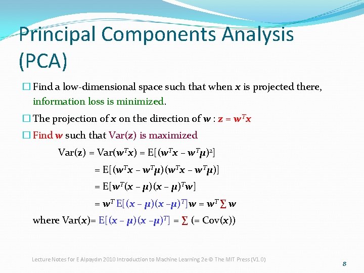
Principal Components Analysis (PCA) � Find a low-dimensional space such that when x is projected there, information loss is minimized. � The projection of x on the direction of w : z = w. Tx � Find w such that Var(z) is maximized Var(z) = Var(w. Tx) = E[(w. Tx – w. Tμ)2] = E[(w. Tx – w. Tμ)] = E[w. T(x – μ)Tw] = w. T E[(x – μ)(x –μ)T]w = w. T ∑ w where Var(x)= E[(x – μ)(x –μ)T] = ∑ (= Cov(x)) Lecture Notes for E Alpaydın 2010 Introduction to Machine Learning 2 e © The MIT Press (V 1. 0) 8

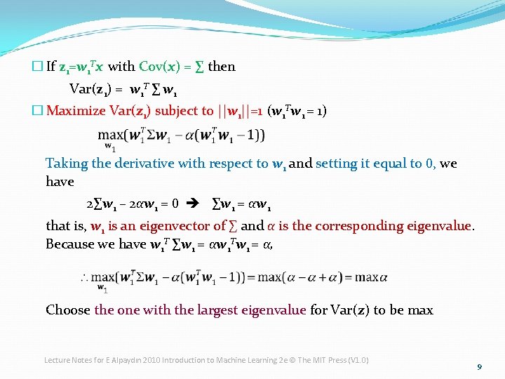
� If z 1=w 1 Tx with Cov(x) = ∑ then Var(z 1) = w 1 T ∑ w 1 � Maximize Var(z 1) subject to ||w 1||=1 (w 1 Tw 1 = 1) Taking the derivative with respect to w 1 and setting it equal to 0, we have 2∑w 1 – 2αw 1 = 0 ∑w 1 = αw 1 that is, w 1 is an eigenvector of ∑ and α is the corresponding eigenvalue. Because we have w 1 T ∑w 1 = αw 1 Tw 1 = α, Choose the one with the largest eigenvalue for Var(z) to be max Lecture Notes for E Alpaydın 2010 Introduction to Machine Learning 2 e © The MIT Press (V 1. 0) 9

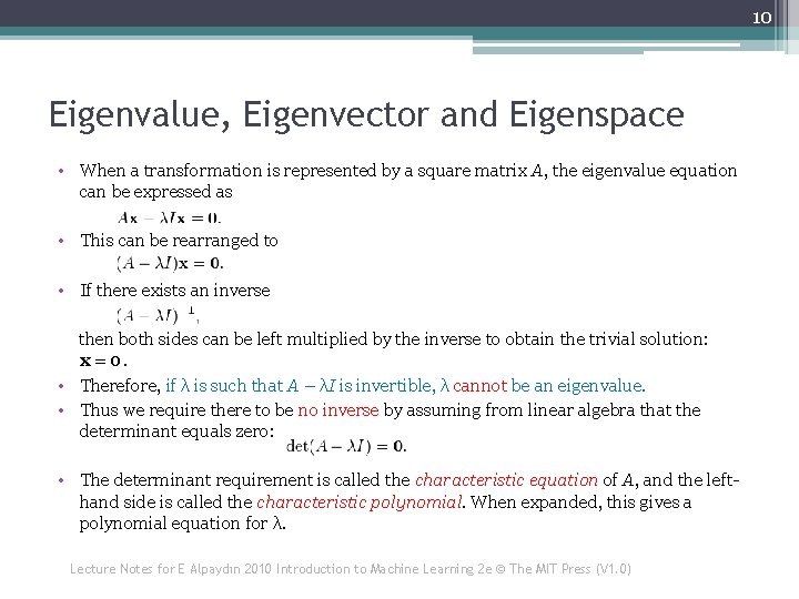
10 Eigenvalue, Eigenvector and Eigenspace • When a transformation is represented by a square matrix A, the eigenvalue equation can be expressed as • This can be rearranged to • If there exists an inverse then both sides can be left multiplied by the inverse to obtain the trivial solution: x = 0. • Therefore, if λ is such that A − λI is invertible, λ cannot be an eigenvalue. • Thus we require there to be no inverse by assuming from linear algebra that the determinant equals zero: • The determinant requirement is called the characteristic equation of A, and the lefthand side is called the characteristic polynomial. When expanded, this gives a polynomial equation for λ. Lecture Notes for E Alpaydın 2010 Introduction to Machine Learning 2 e © The MIT Press (V 1. 0)

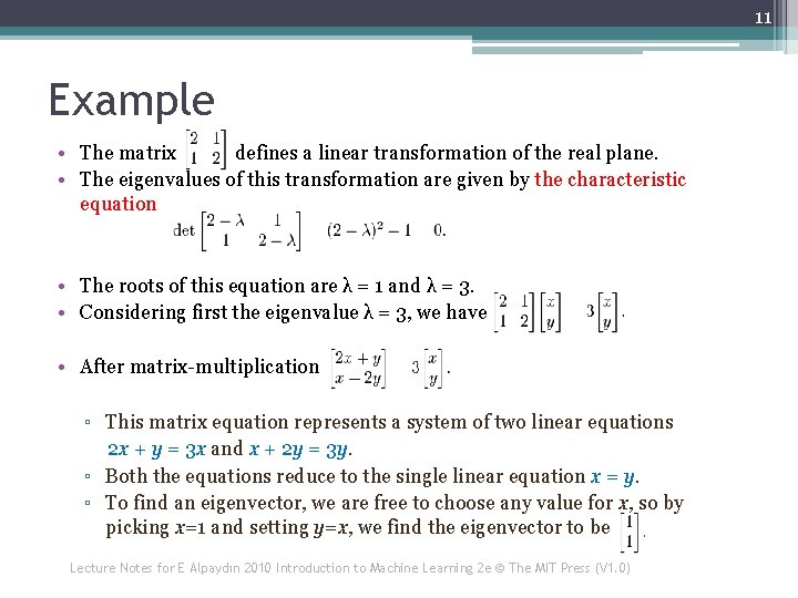
11 Example • The matrix defines a linear transformation of the real plane. • The eigenvalues of this transformation are given by the characteristic equation • The roots of this equation are λ = 1 and λ = 3. • Considering first the eigenvalue λ = 3, we have • After matrix-multiplication ▫ This matrix equation represents a system of two linear equations 2 x + y = 3 x and x + 2 y = 3 y. ▫ Both the equations reduce to the single linear equation x = y. ▫ To find an eigenvector, we are free to choose any value for x, so by picking x=1 and setting y=x, we find the eigenvector to be Lecture Notes for E Alpaydın 2010 Introduction to Machine Learning 2 e © The MIT Press (V 1. 0)

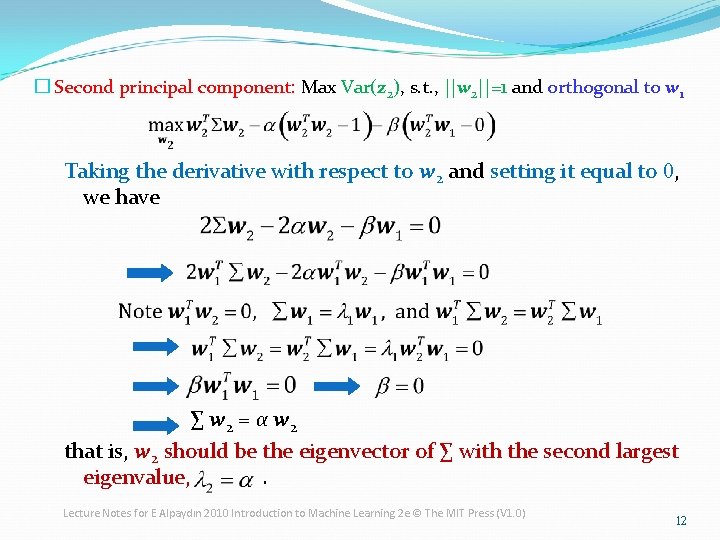
� Second principal component: Max Var(z 2), s. t. , ||w 2||=1 and orthogonal to w 1 Taking the derivative with respect to w 2 and setting it equal to 0, we have ∑ w 2 = α w 2 that is, w 2 should be the eigenvector of ∑ with the second largest eigenvalue, . Lecture Notes for E Alpaydın 2010 Introduction to Machine Learning 2 e © The MIT Press (V 1. 0) 12

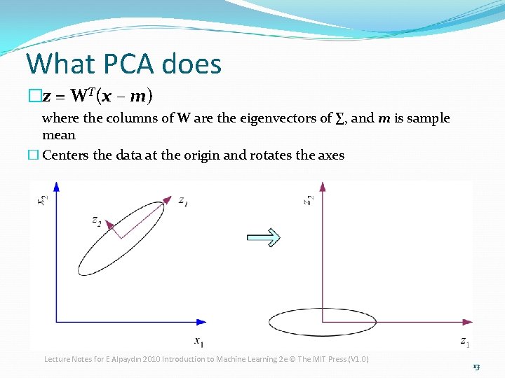
What PCA does �z = WT(x – m) where the columns of W are the eigenvectors of ∑, and m is sample mean � Centers the data at the origin and rotates the axes Lecture Notes for E Alpaydın 2010 Introduction to Machine Learning 2 e © The MIT Press (V 1. 0) 13

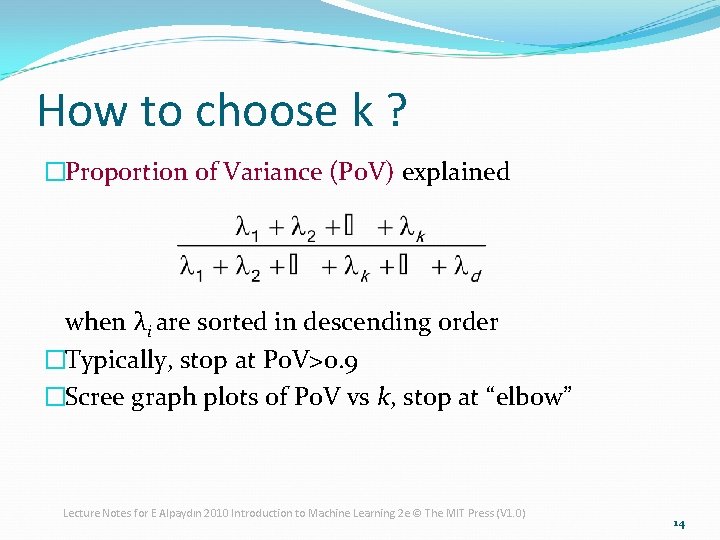
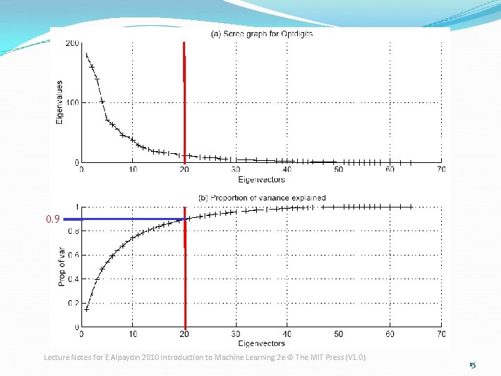
How to choose k ? �Proportion of Variance (Po. V) explained when λi are sorted in descending order �Typically, stop at Po. V>0. 9 �Scree graph plots of Po. V vs k, stop at “elbow” Lecture Notes for E Alpaydın 2010 Introduction to Machine Learning 2 e © The MIT Press (V 1. 0) 14

0. 9 Lecture Notes for E Alpaydın 2010 Introduction to Machine Learning 2 e © The MIT Press (V 1. 0) 15

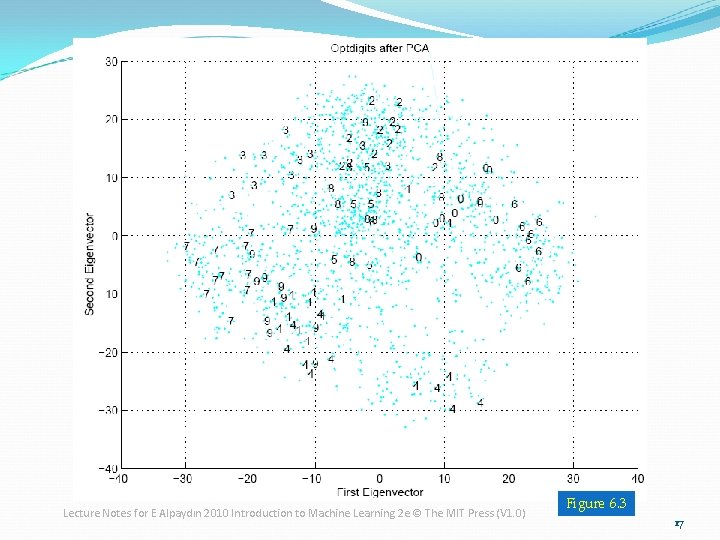
Example of PCA �Figure 6. 3 �Optdigit data plotted in the space of two principal components. �Only the labels of hundred data points are shown to minimize the ink-to-noise ratio. Lecture Notes for E Alpaydın 2010 Introduction to Machine Learning 2 e © The MIT Press (V 1. 0) 16

Lecture Notes for E Alpaydın 2010 Introduction to Machine Learning 2 e © The MIT Press (V 1. 0) Figure 6. 3 17

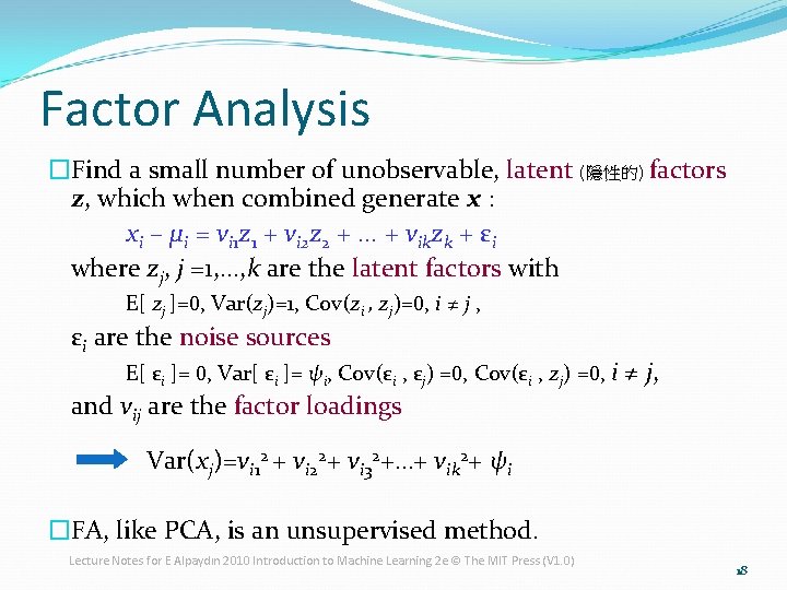
Factor Analysis �Find a small number of unobservable, latent (隱性的) factors z, which when combined generate x : xi – µi = vi 1 z 1 + vi 2 z 2 +. . . + vikzk + εi where zj, j =1, . . . , k are the latent factors with E[ zj ]=0, Var(zj)=1, Cov(zi , zj)=0, i ≠ j , εi are the noise sources E[ εi ]= 0, Var[ εi ]= ψi, Cov(εi , εj) =0, Cov(εi , zj) =0, i ≠ j, and vij are the factor loadings Var(xj)=vi 12 + vi 22+ vi 32+…+ vik 2+ ψi �FA, like PCA, is an unsupervised method. Lecture Notes for E Alpaydın 2010 Introduction to Machine Learning 2 e © The MIT Press (V 1. 0) 18

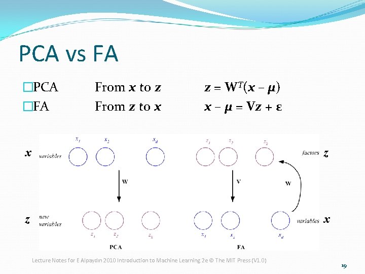
PCA vs FA �PCA �FA From x to z From z to x z = WT(x – µ) x – µ = Vz + ε x z z x Lecture Notes for E Alpaydın 2010 Introduction to Machine Learning 2 e © The MIT Press (V 1. 0) 19

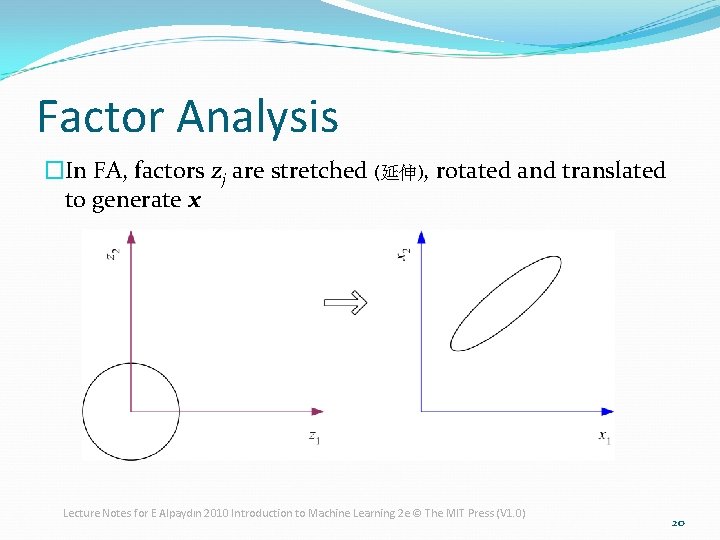
Factor Analysis �In FA, factors zj are stretched (延伸), rotated and translated to generate x Lecture Notes for E Alpaydın 2010 Introduction to Machine Learning 2 e © The MIT Press (V 1. 0) 20

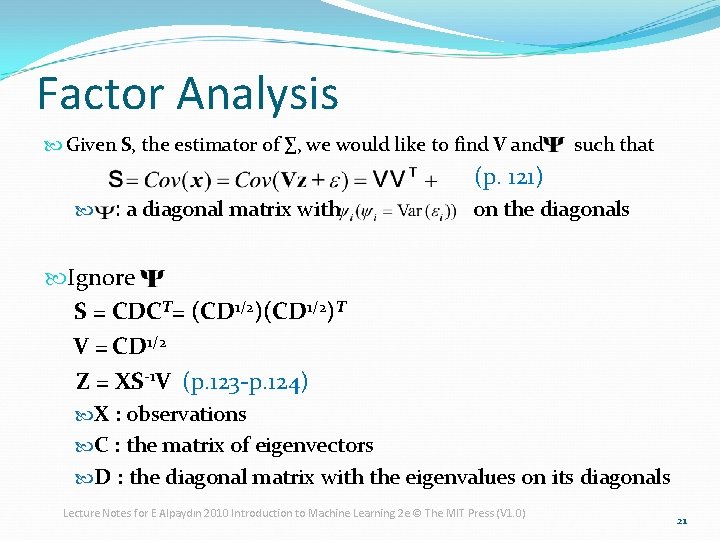
Factor Analysis Given S, the estimator of ∑, we would like to find V and such that (p. 121) : a diagonal matrix with on the diagonals Ignore S = CDCT= (CD 1/2)T V = CD 1/2 Z = XS-1 V (p. 123 -p. 124) X : observations C : the matrix of eigenvectors D : the diagonal matrix with the eigenvalues on its diagonals Lecture Notes for E Alpaydın 2010 Introduction to Machine Learning 2 e © The MIT Press (V 1. 0) 21

22 Example • The following example is a simplification for expository purposes, and should not be taken to be realistic. • Suppose a psychologist proposes a theory that there are two kinds of intelligence, "verbal intelligence" and "mathematical intelligence", neither of which is directly observed. • Evidence for theory is sought in the examination scores from each of 10 different academic fields of 1000 students. • If each student is chosen randomly from a large population, then each student's 10 scores are random variables. • The psychologist's theory may say that for each of the 10 academic fields the score averaged over the group of all students who share some common pair of values for verbal and mathematical "intelligences" is some constant times their level of verbal intelligence plus another constant times their level of mathematical intelligence, i. e. , it is a linear combination of those two "factors". • The numbers for this particular subject, by which the two kinds of intelligence are multiplied to obtain the expected score, are posited by theory to be the same for all intelligence level pairs, and are called "factor loadings" for this subject. Lecture Notes for E Alpaydın 2010 Introduction to Machine Learning 2 e © The MIT Press (V 1. 0)

23 Example • For example, theory may hold that the average student's aptitude(天資) in the field of is {10 × the student's verbal intelligence} + {6 × the student's mathematical intelligence}. • The numbers 10 and 6 are the factor loadings associated with amphibiology (兩棲動 物學). Other academic subjects may have different factor loadings. • Two students having identical degrees of verbal intelligence and identical degrees of mathematical intelligence may have different aptitudes in amphibiology because individual aptitudes differ from average aptitudes. • That difference is called the "error" — a statistical term that means the amount by which an individual differs from what is average for his or her levels of intelligence. • The observable data that go into factor analysis would be 10 scores of each of the 1000 students, a total of 10, 000 numbers. The factor loadings and levels of the two kinds of intelligence of each student must be inferred from the data. (http: //en. wikipedia. org/wiki/Factor_analysis) Lecture Notes for E Alpaydın 2010 Introduction to Machine Learning 2 e © The MIT Press (V 1. 0)

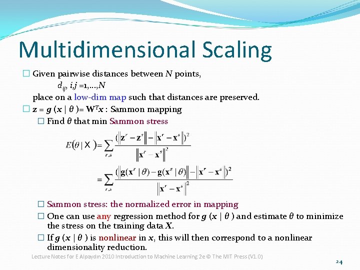
Multidimensional Scaling � Given pairwise distances between N points, dij, i, j =1, . . . , N place on a low-dim map such that distances are preserved. � z = g (x | θ )= WTx : Sammon mapping � Find θ that min Sammon stress � Sammon stress: the normalized error in mapping � One can use any regression method for g (x | θ ) and estimate θ to minimize the stress on the training data X. � If g (x | θ ) is nonlinear in x, this will then correspond to a nonlinear dimensionality reduction. Lecture Notes for E Alpaydın 2010 Introduction to Machine Learning 2 e © The MIT Press (V 1. 0) 24

Map of Europe by MDS Map from CIA – The World Factbook: http: //www. cia. gov/ Lecture Notes for E Alpaydın 2010 Introduction to Machine Learning 2 e © The MIT Press (V 1. 0) 25

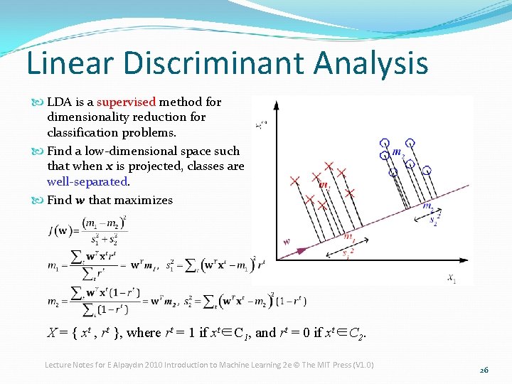
Linear Discriminant Analysis LDA is a supervised method for dimensionality reduction for classification problems. Find a low-dimensional space such that when x is projected, classes are well-separated. Find w that maximizes X = { xt , rt }, where rt = 1 if xt∈C 1, and rt = 0 if xt∈C 2. Lecture Notes for E Alpaydın 2010 Introduction to Machine Learning 2 e © The MIT Press (V 1. 0) 26

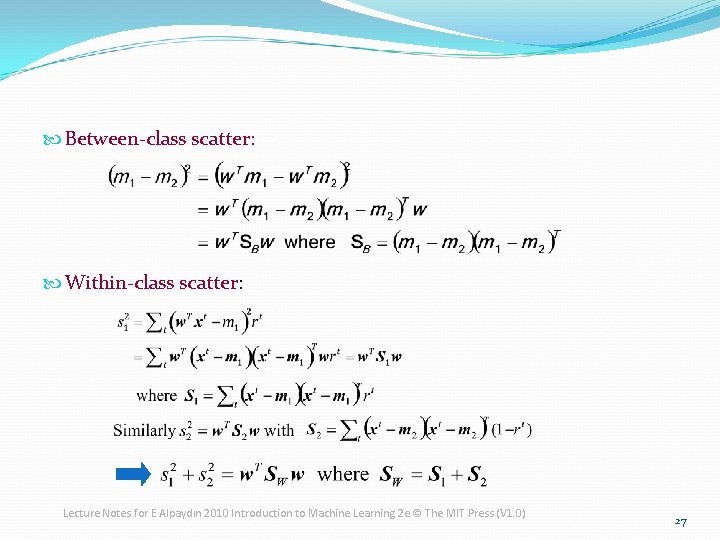
Between-class scatter: Within-class scatter: Lecture Notes for E Alpaydın 2010 Introduction to Machine Learning 2 e © The MIT Press (V 1. 0) 27

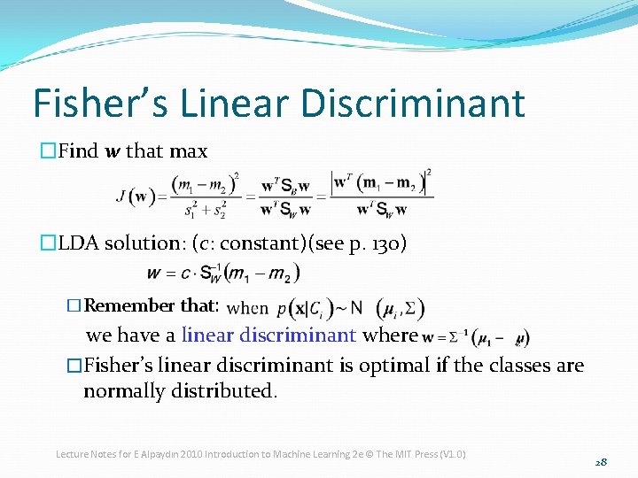
Fisher’s Linear Discriminant �Find w that max �LDA solution: (c: constant)(see p. 130) �Remember that: we have a linear discriminant where �Fisher’s linear discriminant is optimal if the classes are normally distributed. Lecture Notes for E Alpaydın 2010 Introduction to Machine Learning 2 e © The MIT Press (V 1. 0) 28

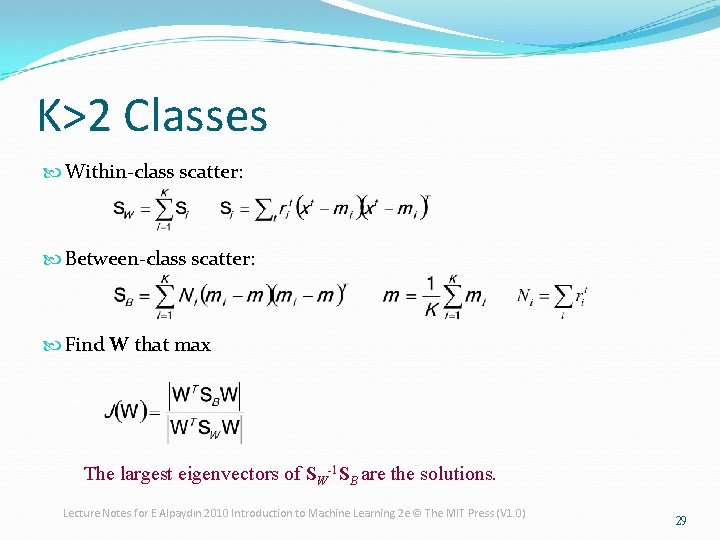
K>2 Classes Within-class scatter: Between-class scatter: Find W that max The largest eigenvectors of SW-1 SB are the solutions. Lecture Notes for E Alpaydın 2010 Introduction to Machine Learning 2 e © The MIT Press (V 1. 0) 29

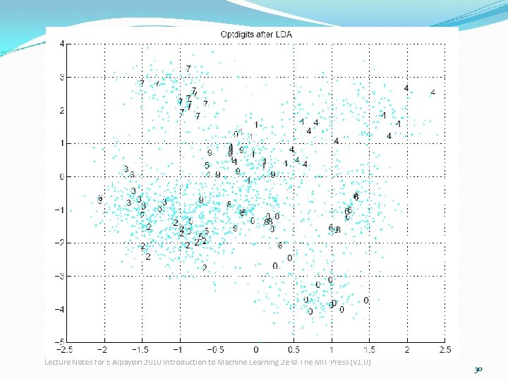
Lecture Notes for E Alpaydın 2010 Introduction to Machine Learning 2 e © The MIT Press (V 1. 0) 30

Exercise �Draw two-class, two-dimensional data such that (a) PCA and LDA find the same direction and (b) PCA and LDA find totally different directions. Lecture Notes for E Alpaydın 2010 Introduction to Machine Learning 2 e © The MIT Press (V 1. 0) 31

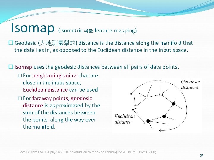
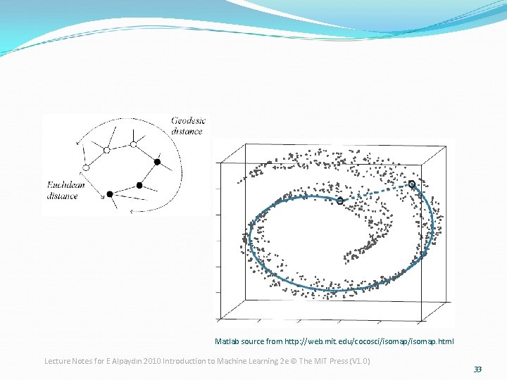
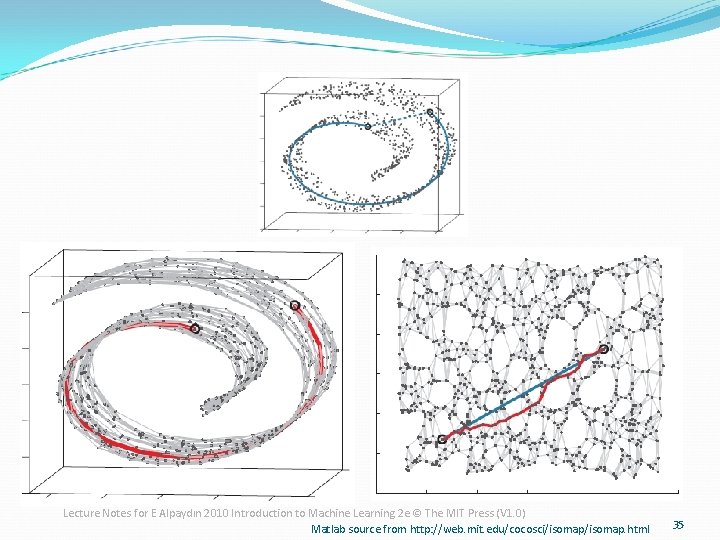
Isomap (Isometric (等量) feature mapping) � Geodesic (大地測量學的) distance is the distance along the manifold that the data lies in, as opposed to the Euclidean distance in the input space. � Isomap uses the geodesic distances between all pairs of data points. � For neighboring points that are close in the input space, Euclidean distance can be used. � For faraway points, geodesic distance is approximated by the sum of the distances between the points along the way over the manifold. Lecture Notes for E Alpaydın 2010 Introduction to Machine Learning 2 e © The MIT Press (V 1. 0) 32

Matlab source from http: //web. mit. edu/cocosci/isomap. html Lecture Notes for E Alpaydın 2010 Introduction to Machine Learning 2 e © The MIT Press (V 1. 0) 33

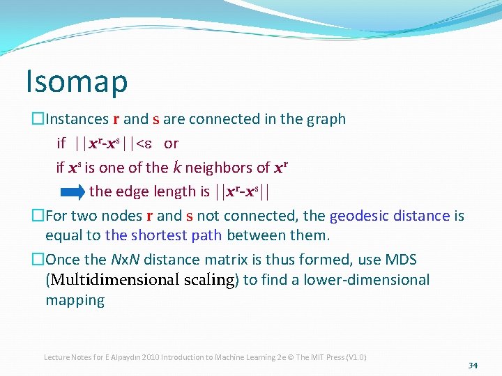
Isomap �Instances r and s are connected in the graph if ||xr-xs||<e or if xs is one of the k neighbors of xr the edge length is ||xr-xs|| �For two nodes r and s not connected, the geodesic distance is equal to the shortest path between them. �Once the Nx. N distance matrix is thus formed, use MDS (Multidimensional scaling) to find a lower-dimensional mapping Lecture Notes for E Alpaydın 2010 Introduction to Machine Learning 2 e © The MIT Press (V 1. 0) 34

Lecture Notes for E Alpaydın 2010 Introduction to Machine Learning 2 e © The MIT Press (V 1. 0) Matlab source from http: //web. mit. edu/cocosci/isomap. html 35

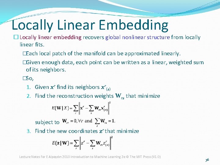
Locally Linear Embedding � Locally linear embedding recovers global nonlinear structure from locally linear fits. �Each local patch of the manifold can be approximated linearly. �Given enough data, each point can be written as a linear, weighted sum of its neighbors. �So, 1. Given xr find its neighbors xr(s) 2. Find the reconstruction weights Wrs that minimize subject to 3. Find the new coordinates zr that minimize Lecture Notes for E Alpaydın 2010 Introduction to Machine Learning 2 e © The MIT Press (V 1. 0) 36

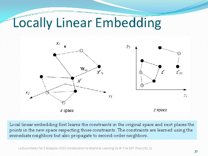
Locally Linear Embedding Local linear embedding first learns the constraints in the original space and next places the points in the new space respecting those constraints. The constraints are learned using the immediate neighbors but also propagate to second-order neighbors. Lecture Notes for E Alpaydın 2010 Introduction to Machine Learning 2 e © The MIT Press (V 1. 0) 37

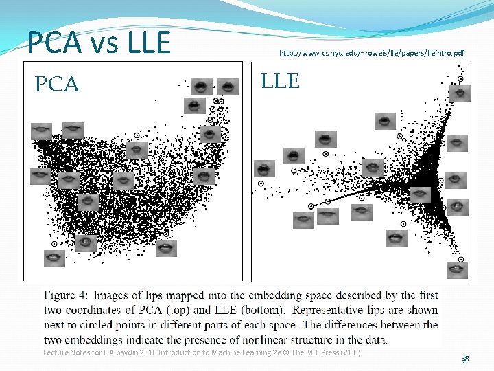
PCA vs LLE PCA http: //www. cs. nyu. edu/~roweis/lle/papers/lleintro. pdf LLE Lecture Notes for E Alpaydın 2010 Introduction to Machine Learning 2 e © The MIT Press (V 1. 0) 38

Exercise �In Isomap, instead of using Euclidean distance, we can also use Mahalanobis distance between neighboring points. What are the advantages and disadvantages of this approach, if any? Lecture Notes for E Alpaydın 2010 Introduction to Machine Learning 2 e © The MIT Press (V 1. 0) 39