Lecture Slides for INTRODUCTION TO Machine Learning 2

Lecture Slides for INTRODUCTION TO Machine Learning 2 nd Edition ETHEM ALPAYDIN © The MIT Press, 2010 alpaydin@boun. edu. tr http: //www. cmpe. boun. edu. tr/~ethem/i 2 ml 2 e

CHAPTER 6: Dimensionality Reduction

Why Reduce Dimensionality? � � � Reduces time complexity: Less computation Reduces space complexity: Less parameters Saves the cost of observing the feature Simpler models are more robust on small datasets More interpretable; simpler explanation Data visualization (structure, groups, outliers, etc) if plotted in 2 or 3 dimensions Lecture Notes for E Alpaydın 2010 Introduction to Machine Learning 2 e © The MIT Press (V 1. 0) 3

Feature Selection vs Extraction �Feature selection: Choosing k<d important features, ignoring the remaining d – k Subset selection algorithms �Feature extraction: Project the original xi , i =1, . . . , d dimensions to new k<d dimensions, zj , j =1, . . . , k Principal components analysis (PCA), linear discriminant analysis (LDA), factor analysis (FA) Lecture Notes for E Alpaydın 2010 Introduction to Machine Learning 2 e © The MIT Press (V 1. 0) 4

Subset Selection �There are 2 d subsets of d features �Forward search: Add the best feature at each step �Set of features F initially Ø. �At each iteration, find the best new feature j = argmini E ( F È xi ) �Add xj to F if E ( F È xj ) < E ( F ) �Hill-climbing O(d 2) algorithm �Backward search: Start with all features and remove one at a time, if possible. �Floating search (Add k, remove l) Lecture Notes for E Alpaydın 2010 Introduction to Machine Learning 2 e © The MIT Press (V 1. 0) 5

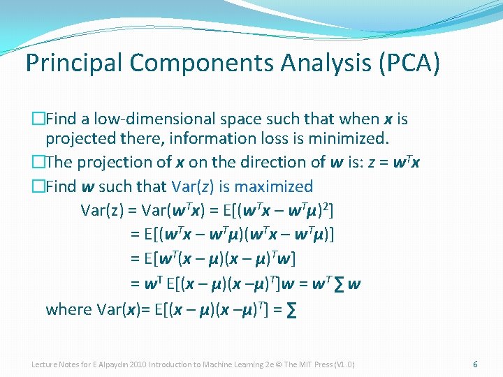
Principal Components Analysis (PCA) �Find a low-dimensional space such that when x is projected there, information loss is minimized. �The projection of x on the direction of w is: z = w. Tx �Find w such that Var(z) is maximized Var(z) = Var(w. Tx) = E[(w. Tx – w. Tμ)2] = E[(w. Tx – w. Tμ)] = E[w. T(x – μ)Tw] = w. T E[(x – μ)(x –μ)T]w = w. T ∑ w where Var(x)= E[(x – μ)(x –μ)T] = ∑ Lecture Notes for E Alpaydın 2010 Introduction to Machine Learning 2 e © The MIT Press (V 1. 0) 6

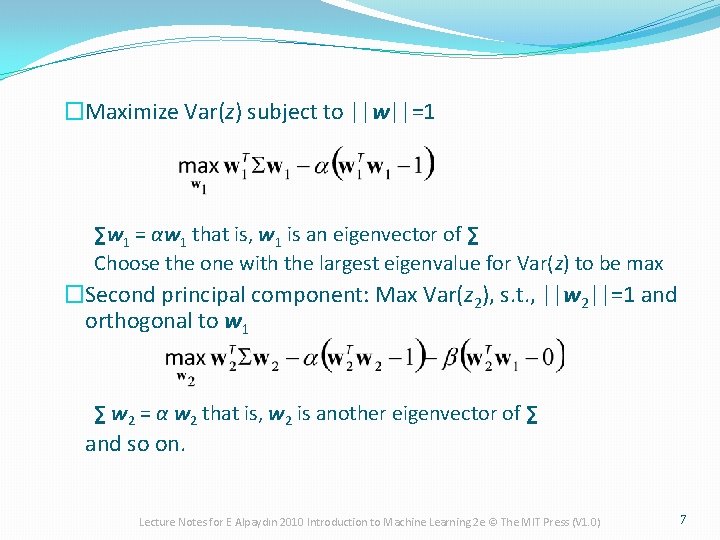
�Maximize Var(z) subject to ||w||=1 ∑w 1 = αw 1 that is, w 1 is an eigenvector of ∑ Choose the one with the largest eigenvalue for Var(z) to be max �Second principal component: Max Var(z 2), s. t. , ||w 2||=1 and orthogonal to w 1 ∑ w 2 = α w 2 that is, w 2 is another eigenvector of ∑ and so on. Lecture Notes for E Alpaydın 2010 Introduction to Machine Learning 2 e © The MIT Press (V 1. 0) 7

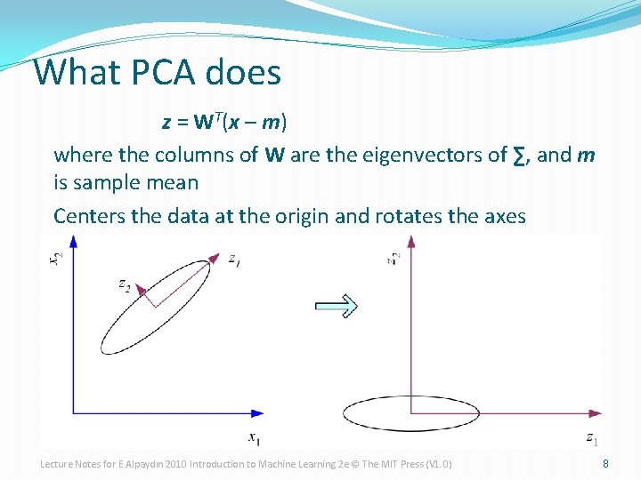
What PCA does z = WT(x – m) where the columns of W are the eigenvectors of ∑, and m is sample mean Centers the data at the origin and rotates the axes Lecture Notes for E Alpaydın 2010 Introduction to Machine Learning 2 e © The MIT Press (V 1. 0) 8

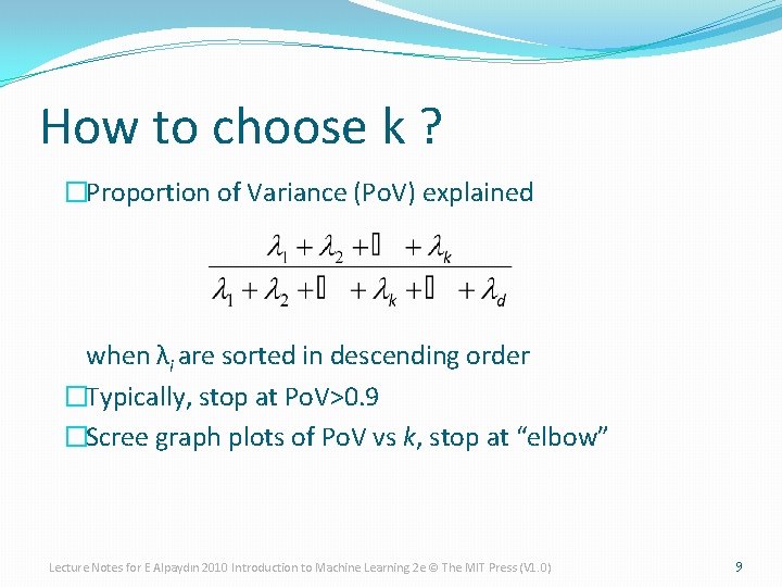
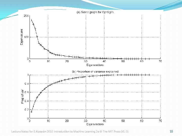
How to choose k ? �Proportion of Variance (Po. V) explained when λi are sorted in descending order �Typically, stop at Po. V>0. 9 �Scree graph plots of Po. V vs k, stop at “elbow” Lecture Notes for E Alpaydın 2010 Introduction to Machine Learning 2 e © The MIT Press (V 1. 0) 9

Lecture Notes for E Alpaydın 2010 Introduction to Machine Learning 2 e © The MIT Press (V 1. 0) 10

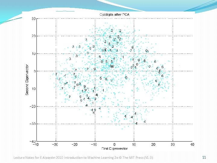
Lecture Notes for E Alpaydın 2010 Introduction to Machine Learning 2 e © The MIT Press (V 1. 0) 11

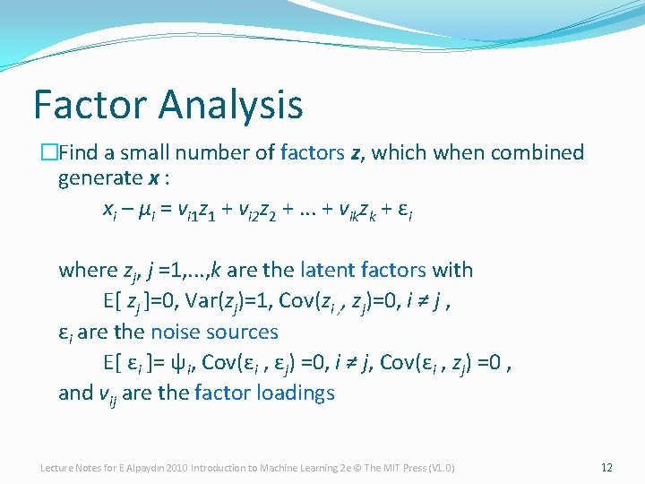
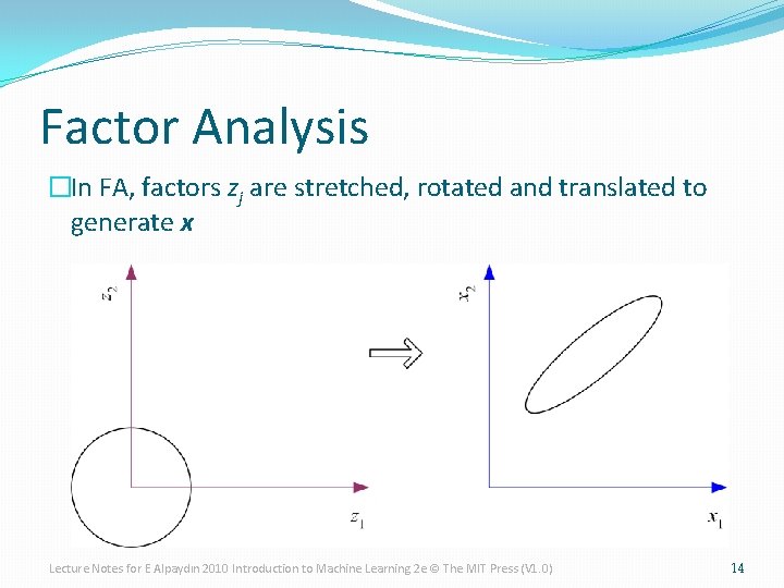
Factor Analysis �Find a small number of factors z, which when combined generate x : xi – µi = vi 1 z 1 + vi 2 z 2 +. . . + vikzk + εi where zj, j =1, . . . , k are the latent factors with E[ zj ]=0, Var(zj)=1, Cov(zi , , zj)=0, i ≠ j , εi are the noise sources E[ εi ]= ψi, Cov(εi , εj) =0, i ≠ j, Cov(εi , zj) =0 , and vij are the factor loadings Lecture Notes for E Alpaydın 2010 Introduction to Machine Learning 2 e © The MIT Press (V 1. 0) 12

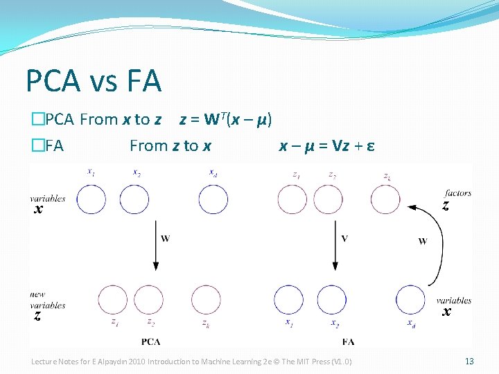
PCA vs FA �PCA From x to z z = WT(x – µ) �FA From z to x x – µ = Vz + ε x z z x Lecture Notes for E Alpaydın 2010 Introduction to Machine Learning 2 e © The MIT Press (V 1. 0) 13

Factor Analysis �In FA, factors zj are stretched, rotated and translated to generate x Lecture Notes for E Alpaydın 2010 Introduction to Machine Learning 2 e © The MIT Press (V 1. 0) 14

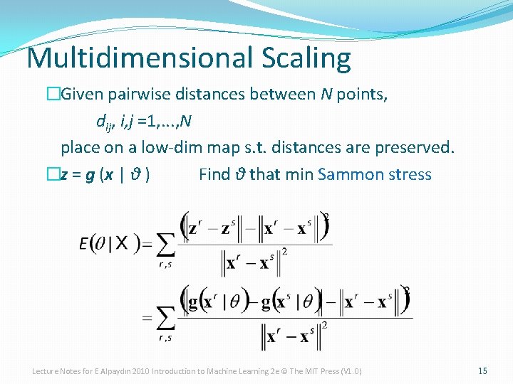
Multidimensional Scaling �Given pairwise distances between N points, dij, i, j =1, . . . , N place on a low-dim map s. t. distances are preserved. �z = g (x | θ ) Find θ that min Sammon stress Lecture Notes for E Alpaydın 2010 Introduction to Machine Learning 2 e © The MIT Press (V 1. 0) 15

Map of Europe by MDS Map from CIA – The World Factbook: http: //www. cia. gov/ Lecture Notes for E Alpaydın 2010 Introduction to Machine Learning 2 e © The MIT Press (V 1. 0) 16

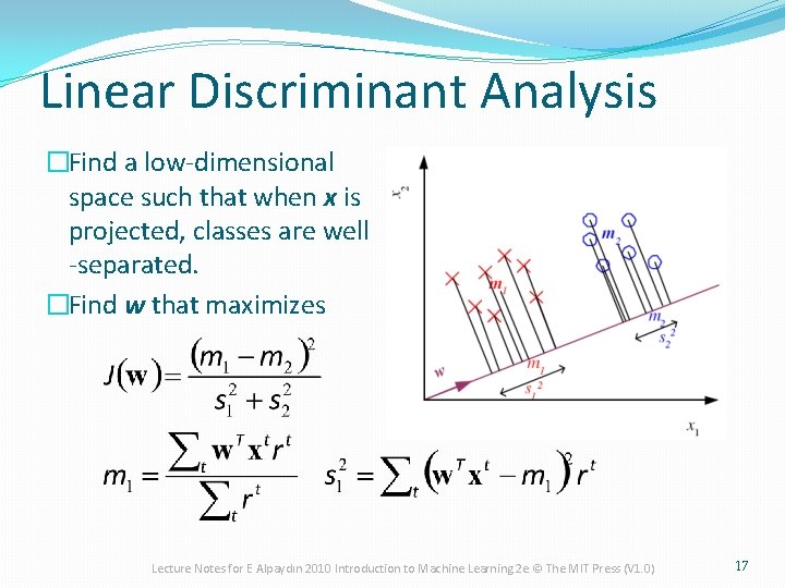
Linear Discriminant Analysis �Find a low-dimensional space such that when x is projected, classes are well -separated. �Find w that maximizes Lecture Notes for E Alpaydın 2010 Introduction to Machine Learning 2 e © The MIT Press (V 1. 0) 17

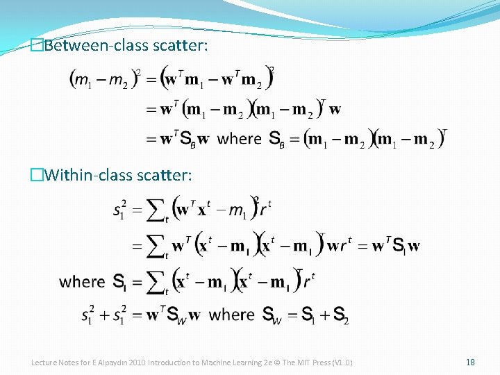
�Between-class scatter: �Within-class scatter: Lecture Notes for E Alpaydın 2010 Introduction to Machine Learning 2 e © The MIT Press (V 1. 0) 18

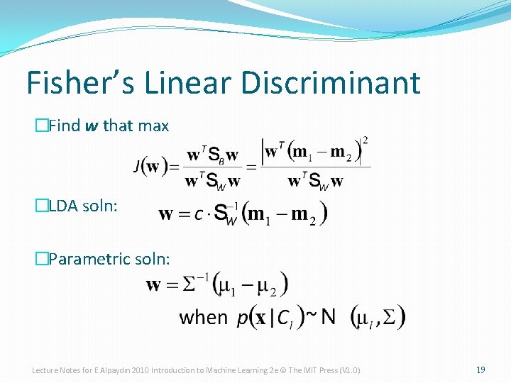
Fisher’s Linear Discriminant �Find w that max �LDA soln: �Parametric soln: Lecture Notes for E Alpaydın 2010 Introduction to Machine Learning 2 e © The MIT Press (V 1. 0) 19

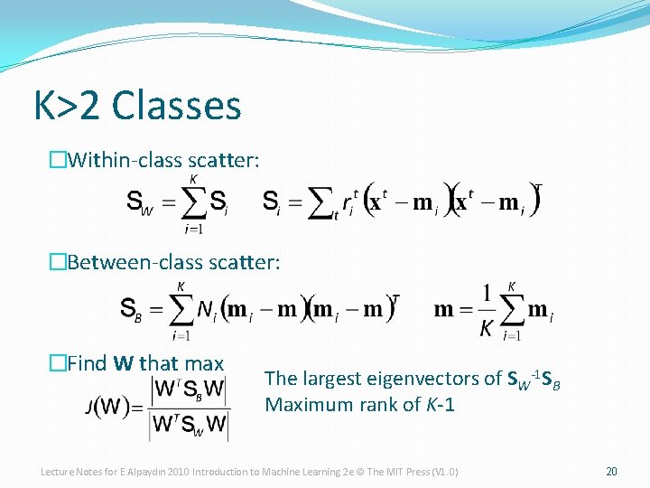
K>2 Classes �Within-class scatter: �Between-class scatter: �Find W that max The largest eigenvectors of SW-1 SB Maximum rank of K-1 Lecture Notes for E Alpaydın 2010 Introduction to Machine Learning 2 e © The MIT Press (V 1. 0) 20

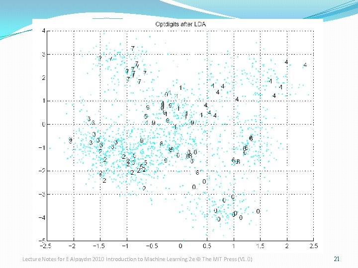
Lecture Notes for E Alpaydın 2010 Introduction to Machine Learning 2 e © The MIT Press (V 1. 0) 21

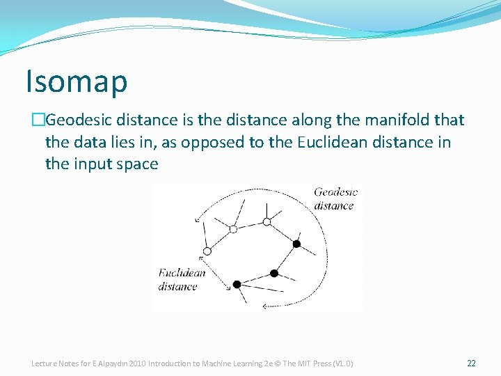
Isomap �Geodesic distance is the distance along the manifold that the data lies in, as opposed to the Euclidean distance in the input space Lecture Notes for E Alpaydın 2010 Introduction to Machine Learning 2 e © The MIT Press (V 1. 0) 22

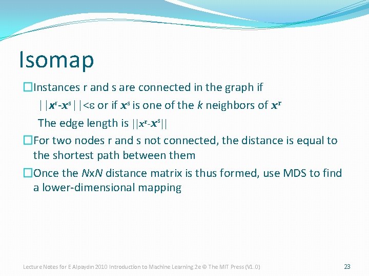
Isomap �Instances r and s are connected in the graph if ||xr-xs||<e or if xs is one of the k neighbors of xr The edge length is ||xr-xs|| �For two nodes r and s not connected, the distance is equal to the shortest path between them �Once the Nx. N distance matrix is thus formed, use MDS to find a lower-dimensional mapping Lecture Notes for E Alpaydın 2010 Introduction to Machine Learning 2 e © The MIT Press (V 1. 0) 23

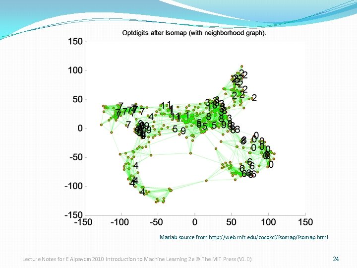
Matlab source from http: //web. mit. edu/cocosci/isomap. html Lecture Notes for E Alpaydın 2010 Introduction to Machine Learning 2 e © The MIT Press (V 1. 0) 24

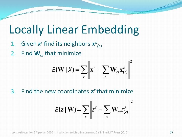
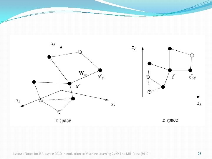
Locally Linear Embedding 1. Given xr find its neighbors xs(r) 2. Find Wrs that minimize 3. Find the new coordinates zr that minimize Lecture Notes for E Alpaydın 2010 Introduction to Machine Learning 2 e © The MIT Press (V 1. 0) 25

Lecture Notes for E Alpaydın 2010 Introduction to Machine Learning 2 e © The MIT Press (V 1. 0) 26

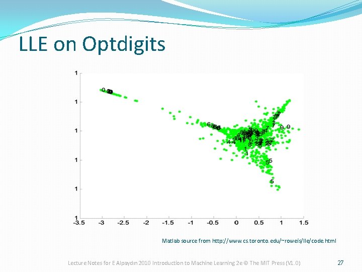
LLE on Optdigits Matlab source from http: //www. cs. toronto. edu/~roweis/lle/code. html Lecture Notes for E Alpaydın 2010 Introduction to Machine Learning 2 e © The MIT Press (V 1. 0) 27