Lecture Slides for INTRODUCTION TO Machine Learning 2

Lecture Slides for INTRODUCTION TO Machine Learning 2 nd Edition ETHEM ALPAYDIN © The MIT Press, 2010 alpaydin@boun. edu. tr http: //www. cmpe. boun. edu. tr/~ethem/i 2 ml 2 e

CHAPTER 4: Parametric Methods

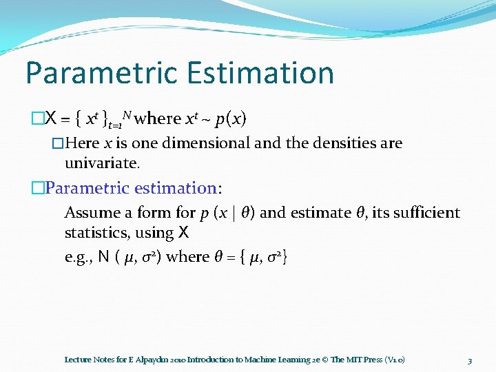
Parametric Estimation �X = { xt }t=1 N where xt ~ p(x) �Here x is one dimensional and the densities are univariate. �Parametric estimation: Assume a form for p (x | θ) and estimate θ, its sufficient statistics, using X e. g. , N ( μ, σ2) where θ = { μ, σ2} Lecture Notes for E Alpaydın 2010 Introduction to Machine Learning 2 e © The MIT Press (V 1. 0) 3

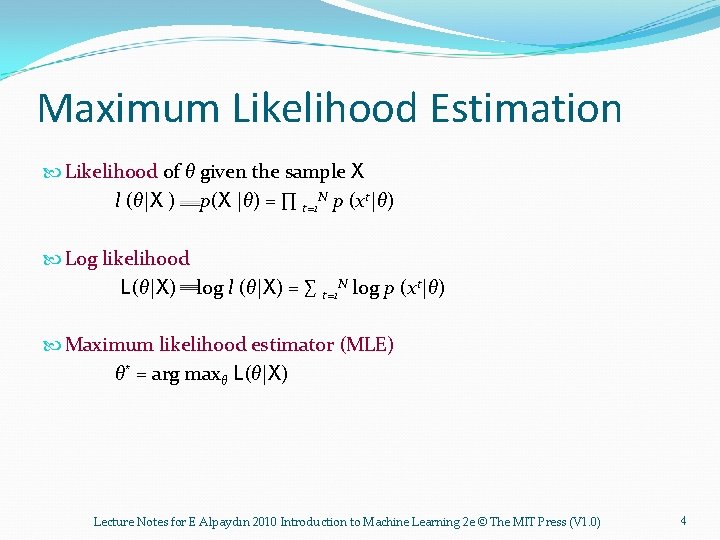
Maximum Likelihood Estimation Likelihood of θ given the sample X l (θ|X ) p(X |θ) = ∏ t=1 N p (xt|θ) Log likelihood L(θ|X) log l (θ|X) = ∑ t=1 N log p (xt|θ) Maximum likelihood estimator (MLE) θ* = arg maxθ L(θ|X) Lecture Notes for E Alpaydın 2010 Introduction to Machine Learning 2 e © The MIT Press (V 1. 0) 4

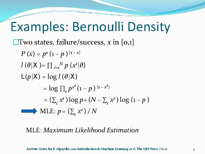
Examples: Bernoulli Density �Two states, failure/success, x in {0, 1} P (x) = px (1 – p ) (1 – x) l (θ|X )= ∏ t=1 N p (xt|θ) L(p|X) = log l (θ|X) = log ∏t pxt (1 – p ) (1 – xt) = (∑t xt ) log p+ (N – ∑t xt ) log (1 – p ) MLE: p = (∑t xt ) / N MLE: Maximum Likelihood Estimation Lecture Notes for E Alpaydın 2010 Introduction to Machine Learning 2 e © The MIT Press (V 1. 0) 5

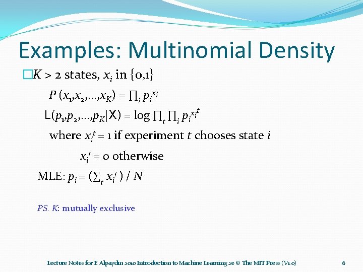
Examples: Multinomial Density �K > 2 states, xi in {0, 1} P (x 1, x 2, . . . , x. K) = ∏i pixi L(p 1, p 2, . . . , p. K|X) = log ∏t ∏i pixit where xit = 1 if experiment t chooses state i xit = 0 otherwise MLE: pi = (∑t xit ) / N PS. K: mutually exclusive Lecture Notes for E Alpaydın 2010 Introduction to Machine Learning 2 e © The MIT Press (V 1. 0) 6

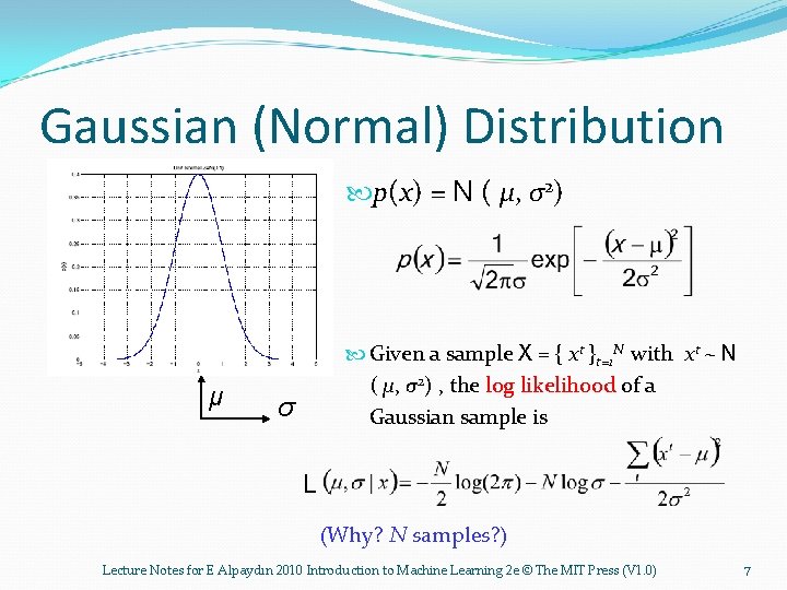
Gaussian (Normal) Distribution p(x) = N ( μ, σ2) μ Given a sample X = { xt }t=1 N with xt ~ N ( μ, σ2) , the log likelihood of a Gaussian sample is σ L (Why? N samples? ) Lecture Notes for E Alpaydın 2010 Introduction to Machine Learning 2 e © The MIT Press (V 1. 0) 7

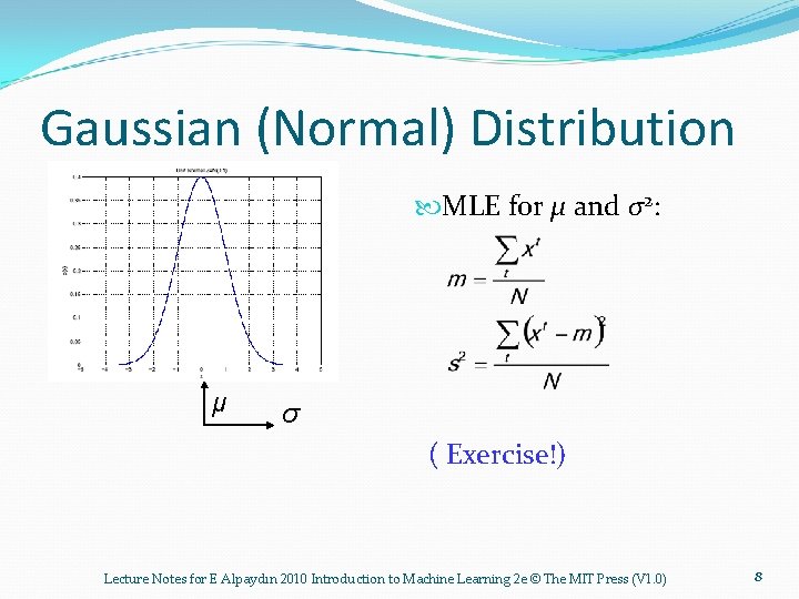
Gaussian (Normal) Distribution MLE for μ and σ2: μ σ ( Exercise!) Lecture Notes for E Alpaydın 2010 Introduction to Machine Learning 2 e © The MIT Press (V 1. 0) 8

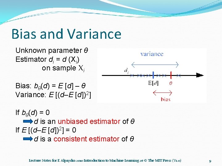
Bias and Variance Unknown parameter θ Estimator di = d (Xi) on sample Xi Bias: bθ(d) = E [d] – θ Variance: E [(d–E [d])2] θ If bθ(d) = 0 d is an unbiased estimator of θ If E [(d–E [d])2] = 0 d is a consistent estimator of θ Lecture Notes for E Alpaydın 2010 Introduction to Machine Learning 2 e © The MIT Press (V 1. 0) 9

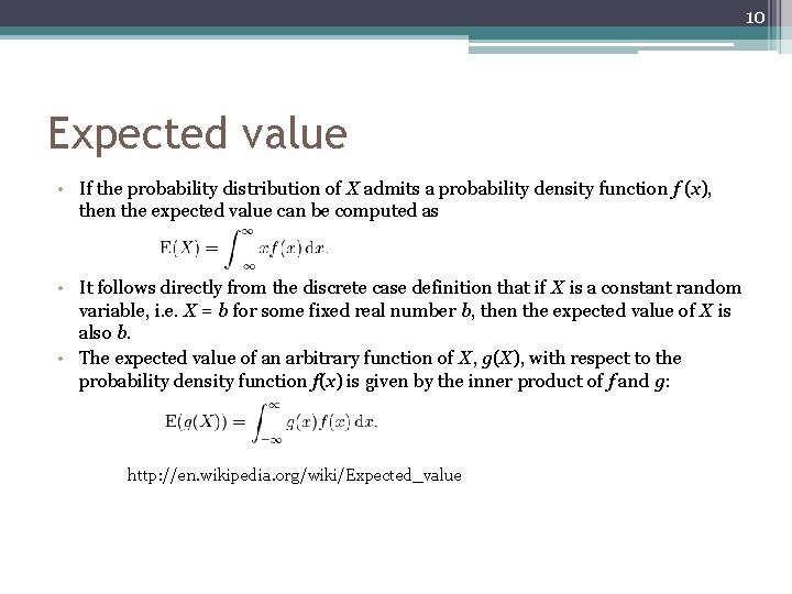
10 Expected value • If the probability distribution of X admits a probability density function f (x), then the expected value can be computed as • It follows directly from the discrete case definition that if X is a constant random variable, i. e. X = b for some fixed real number b, then the expected value of X is also b. • The expected value of an arbitrary function of X, g(X), with respect to the probability density function f(x) is given by the inner product of f and g: http: //en. wikipedia. org/wiki/Expected_value

Bias and Variance For example: Var [m] 0 as N ∞ m is also a consistent estimator Lecture Notes for E Alpaydın 2010 Introduction to Machine Learning 2 e © The MIT Press (V 1. 0) 11

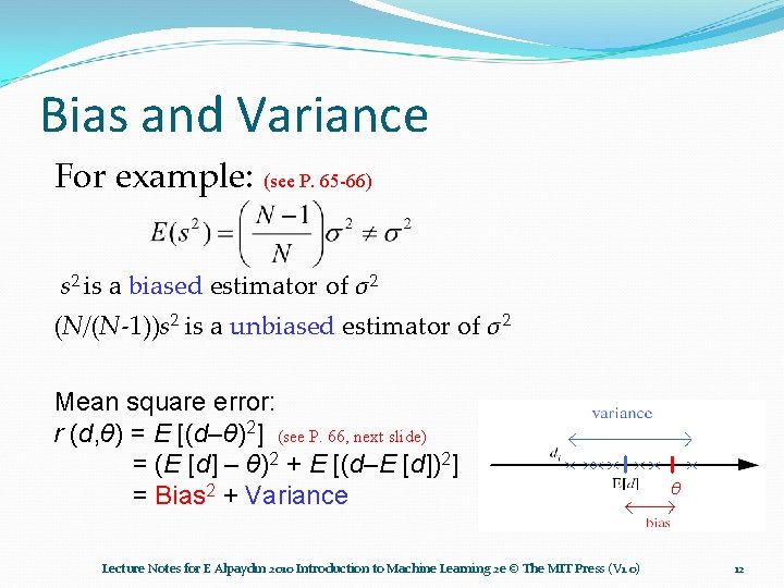
Bias and Variance For example: (see P. 65 -66) s 2 is a biased estimator of σ2 (N/(N-1))s 2 is a unbiased estimator of σ2 Mean square error: r (d, θ) = E [(d–θ)2] (see P. 66, next slide) = (E [d] – θ)2 + E [(d–E [d])2] = Bias 2 + Variance Lecture Notes for E Alpaydın 2010 Introduction to Machine Learning 2 e © The MIT Press (V 1. 0) θ 12

Bias and Variance Lecture Notes for E Alpaydın 2010 Introduction to Machine Learning 2 e © The MIT Press (V 1. 0) 13

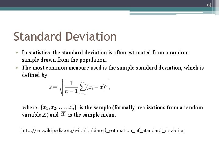
14 Standard Deviation • In statistics, the standard deviation is often estimated from a random sample drawn from the population. • The most common measure used is the sample standard deviation, which is defined by where variable X) and is the sample (formally, realizations from a random is the sample mean. http: //en. wikipedia. org/wiki/Unbiased_estimation_of_standard_deviation

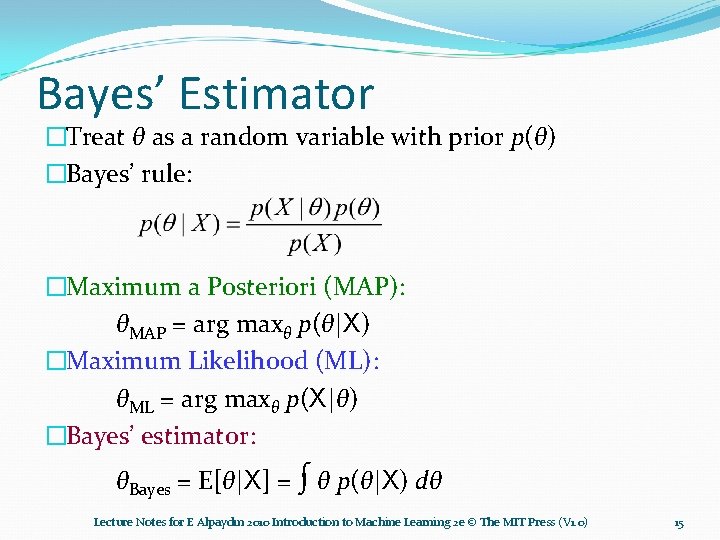
Bayes’ Estimator �Treat θ as a random variable with prior p(θ) �Bayes’ rule: �Maximum a Posteriori (MAP): θMAP = arg maxθ p(θ|X) �Maximum Likelihood (ML): θML = arg maxθ p(X|θ) �Bayes’ estimator: θBayes = E[θ|X] = ∫ θ p(θ|X) dθ Lecture Notes for E Alpaydın 2010 Introduction to Machine Learning 2 e © The MIT Press (V 1. 0) 15

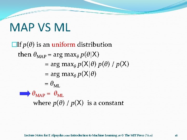
MAP VS ML �If p(θ) is an uniform distribution then θMAP = arg maxθ p(θ|X) = arg maxθ p(X|θ) p(θ) / p(X) = arg maxθ p(X|θ) = θML θMAP = θML where p(θ) / p(X) is a constant Lecture Notes for E Alpaydın 2010 Introduction to Machine Learning 2 e © The MIT Press (V 1. 0) 16

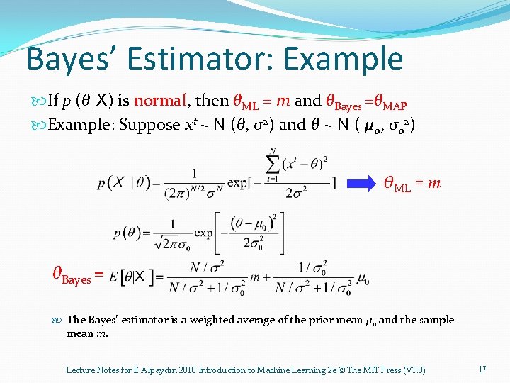
Bayes’ Estimator: Example If p (θ|X) is normal, then θML = m and θBayes =θMAP Example: Suppose xt ~ N (θ, σ2) and θ ~ N ( μ 0, σ02) θML = m θBayes = The Bayes’ estimator is a weighted average of the prior mean μ 0 and the sample mean m. Lecture Notes for E Alpaydın 2010 Introduction to Machine Learning 2 e © The MIT Press (V 1. 0) 17

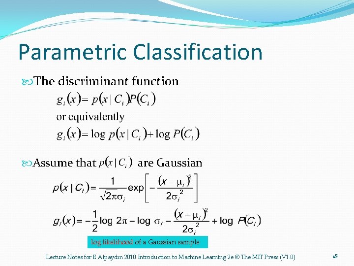
Parametric Classification The discriminant function Assume that are Gaussian log likelihood of a Gaussian sample Lecture Notes for E Alpaydın 2010 Introduction to Machine Learning 2 e © The MIT Press (V 1. 0) 18

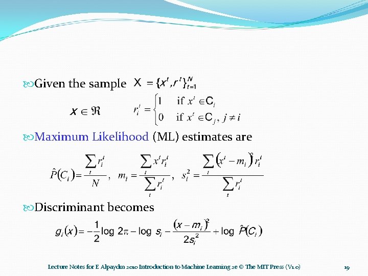
Given the sample Maximum Likelihood (ML) estimates are Discriminant becomes Lecture Notes for E Alpaydın 2010 Introduction to Machine Learning 2 e © The MIT Press (V 1. 0) 19

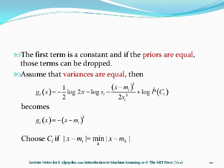
The first term is a constant and if the priors are equal, those terms can be dropped. Assume that variances are equal, then becomes Choose Ci if Lecture Notes for E Alpaydın 2010 Introduction to Machine Learning 2 e © The MIT Press (V 1. 0) 20

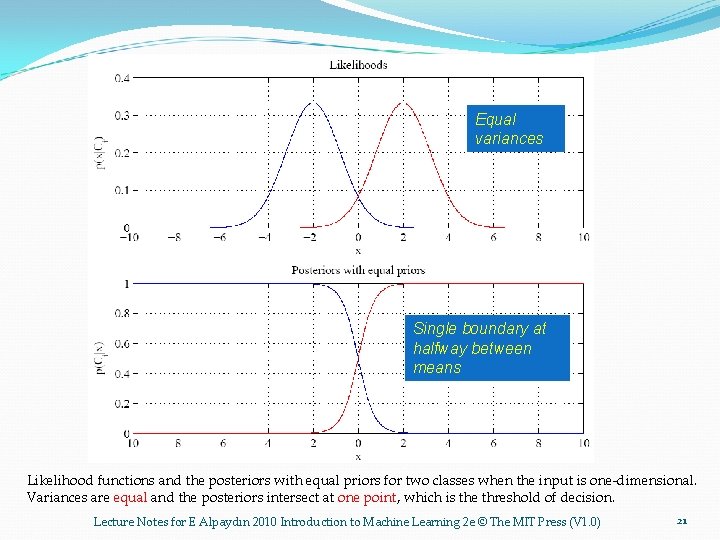
Equal variances Single boundary at halfway between means Likelihood functions and the posteriors with equal priors for two classes when the input is one-dimensional. Variances are equal and the posteriors intersect at one point, which is the threshold of decision. Lecture Notes for E Alpaydın 2010 Introduction to Machine Learning 2 e © The MIT Press (V 1. 0) 21

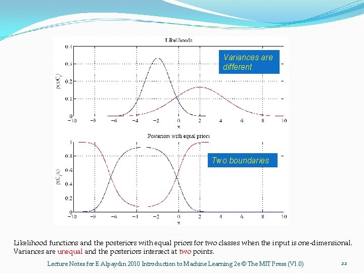
Variances are different Two boundaries Likelihood functions and the posteriors with equal priors for two classes when the input is one-dimensional. Variances are unequal and the posteriors intersect at two points. Lecture Notes for E Alpaydın 2010 Introduction to Machine Learning 2 e © The MIT Press (V 1. 0) 22

Exercise �For a two-class problem, generate normal samples for two classes with different variances, then use parametric classification to estimate the discriminant points. Compare these with theoretical values. PS. You can use normal sample generation tools. Lecture Notes for E Alpaydın 2010 Introduction to Machine Learning 2 e © The MIT Press (V 1. 0) 23

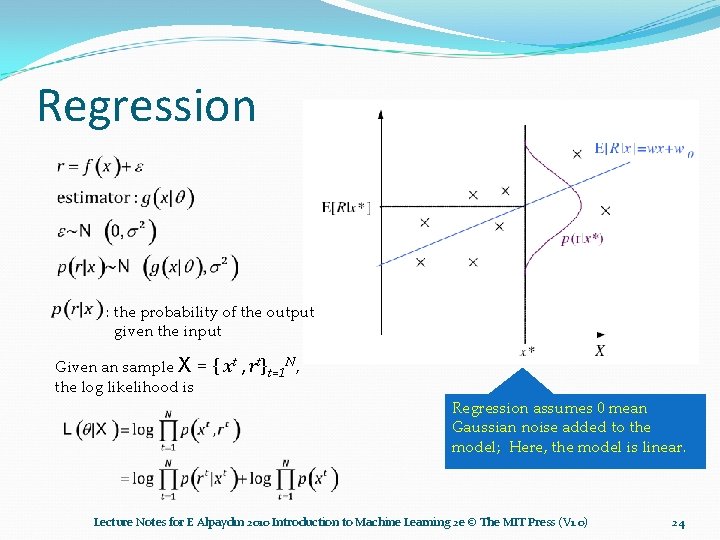
Regression : the probability of the output given the input Given an sample X = the log likelihood is { xt , rt}t=1 N, Regression assumes 0 mean Gaussian noise added to the model; Here, the model is linear. Lecture Notes for E Alpaydın 2010 Introduction to Machine Learning 2 e © The MIT Press (V 1. 0) 24

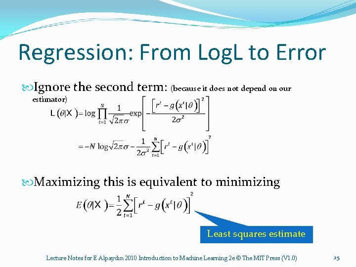
Regression: From Log. L to Error Ignore the second term: (because it does not depend on our estimator) Maximizing this is equivalent to minimizing Least squares estimate Lecture Notes for E Alpaydın 2010 Introduction to Machine Learning 2 e © The MIT Press (V 1. 0) 25

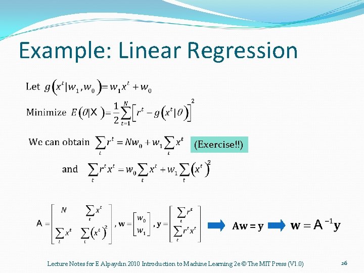
Example: Linear Regression (Exercise!!) Lecture Notes for E Alpaydın 2010 Introduction to Machine Learning 2 e © The MIT Press (V 1. 0) 26

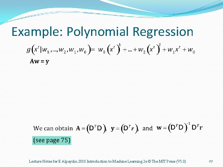
Example: Polynomial Regression Lecture Notes for E Alpaydın 2010 Introduction to Machine Learning 2 e © The MIT Press (V 1. 0) 27

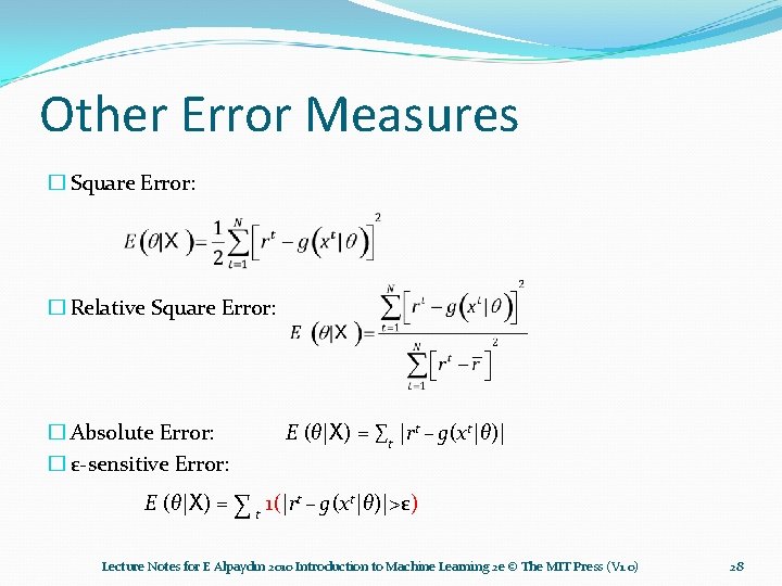
Other Error Measures � Square Error: � Relative Square Error: � Absolute Error: � ε-sensitive Error: E (θ|X) = ∑t |rt – g(xt|θ)| E (θ|X) = ∑ t 1(|rt – g(xt|θ)|>ε) Lecture Notes for E Alpaydın 2010 Introduction to Machine Learning 2 e © The MIT Press (V 1. 0) 28

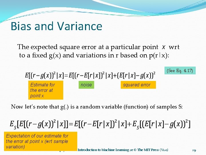
Bias and Variance The expected square error at a particular point x wrt to a fixed g(x) and variations in r based on p(r|x): (See Eq. 4. 17) Estimate for the error at point x noise squared error Now let’s note that g(. ) is a random variable (function) of samples S: Expectation of our estimate for the error at point x (wrt sample variation) Lecture Notes for E Alpaydın 2010 Introduction to Machine Learning 2 e © The MIT Press (V 1. 0) 29

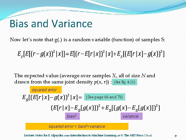
Bias and Variance Now let’s note that g(. ) is a random variable (function) of samples S: The expected value (average over samples X, all of size N and drawn from the same joint density p(x, r)) : (See Eq. 4. 11) squared error (See page 66 and 76) bias 2 variance squared error = bais 2+variance Lecture Notes for E Alpaydın 2010 Introduction to Machine Learning 2 e © The MIT Press (V 1. 0) 31

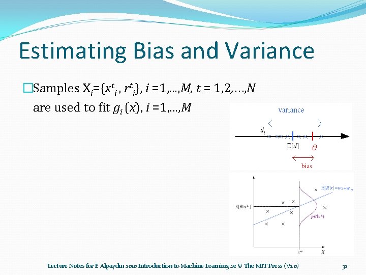
Estimating Bias and Variance �Samples Xi={xti , rti}, i =1, . . . , M, t = 1, 2, …, N are used to fit gi (x), i =1, . . . , M θ Lecture Notes for E Alpaydın 2010 Introduction to Machine Learning 2 e © The MIT Press (V 1. 0) 32

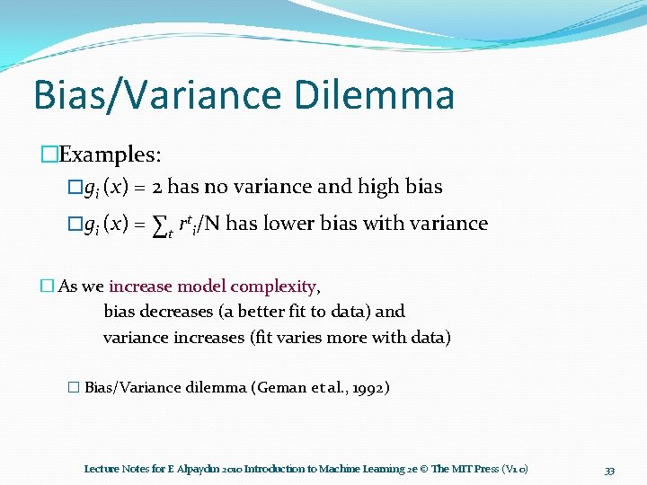
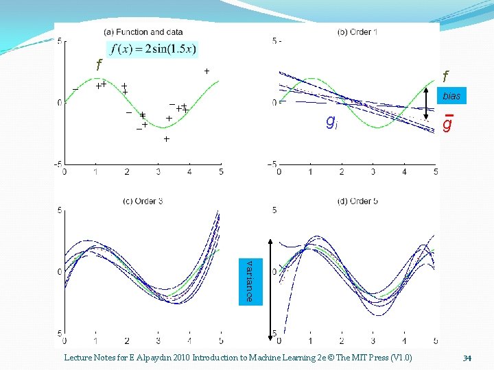
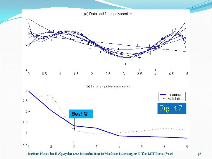
Bias/Variance Dilemma �Examples: �gi (x) = 2 has no variance and high bias �gi (x) = ∑t rti/N has lower bias with variance � As we increase model complexity, bias decreases (a better fit to data) and variance increases (fit varies more with data) � Bias/Variance dilemma (Geman et al. , 1992) Lecture Notes for E Alpaydın 2010 Introduction to Machine Learning 2 e © The MIT Press (V 1. 0) 33

f f bias gi g variance Lecture Notes for E Alpaydın 2010 Introduction to Machine Learning 2 e © The MIT Press (V 1. 0) 34

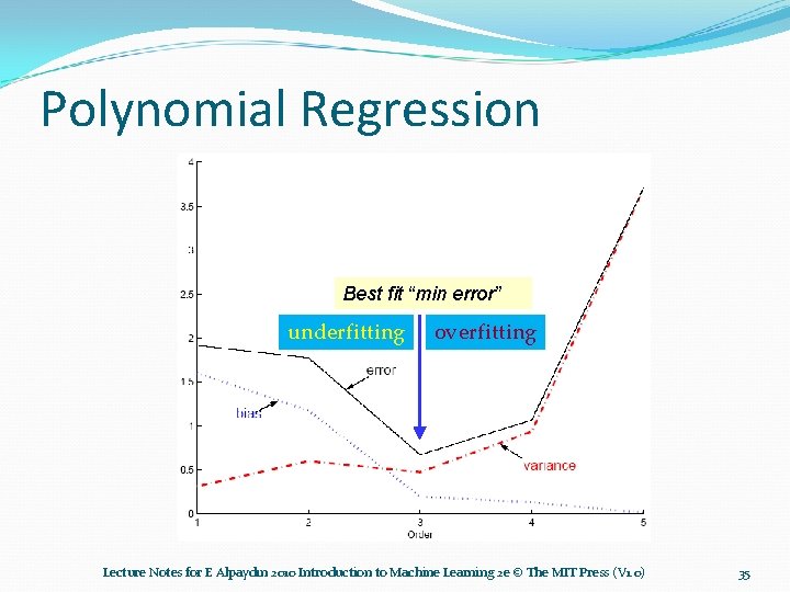
Polynomial Regression Best fit “min error” underfitting overfitting Lecture Notes for E Alpaydın 2010 Introduction to Machine Learning 2 e © The MIT Press (V 1. 0) 35

Best fit, Fig. 4. 7 Lecture Notes for E Alpaydın 2010 Introduction to Machine Learning 2 e © The MIT Press (V 1. 0) 36

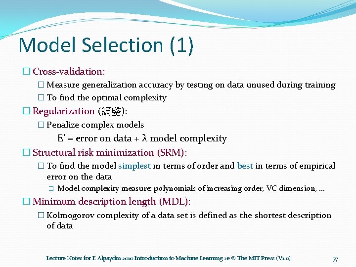
Model Selection (1) � Cross-validation: � Measure generalization accuracy by testing on data unused during training � To find the optimal complexity � Regularization (調整): � Penalize complex models E’ = error on data + λ model complexity � Structural risk minimization (SRM): � To find the model simplest in terms of order and best in terms of empirical error on the data � Model complexity measure: polynomials of increasing order, VC dimension, . . . � Minimum description length (MDL): � Kolmogorov complexity of a data set is defined as the shortest description of data Lecture Notes for E Alpaydın 2010 Introduction to Machine Learning 2 e © The MIT Press (V 1. 0) 37

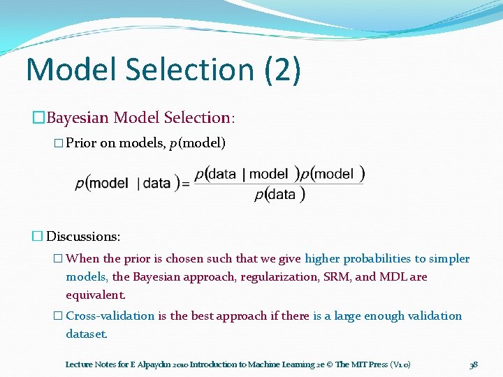
Model Selection (2) �Bayesian Model Selection: � Prior on models, p(model) � Discussions: � When the prior is chosen such that we give higher probabilities to simpler models, the Bayesian approach, regularization, SRM, and MDL are equivalent. � Cross-validation is the best approach if there is a large enough validation dataset. Lecture Notes for E Alpaydın 2010 Introduction to Machine Learning 2 e © The MIT Press (V 1. 0) 38

Regression example Coefficients increase in magnitude as order increases: 1: [-0. 0769, 0. 0016] 2: [0. 1682, -0. 6657, 0. 0080] 3: [0. 4238, -2. 5778, 3. 4675, -0. 0002 4: [-0. 1093, 1. 4356, -5. 5007, 6. 0454, -0. 0019] Please compare with Fig. 4. 5, p. 78. Lecture Notes for E Alpaydın 2010 Introduction to Machine Learning 2 e © The MIT Press (V 1. 0) 39