Lecture Slides for INTRODUCTION TO Machine Learning 2

Lecture Slides for INTRODUCTION TO Machine Learning 2 nd Edition ETHEM ALPAYDIN © The MIT Press, 2010 alpaydin@boun. edu. tr http: //www. cmpe. boun. edu. tr/~ethem/i 2 ml 2 e

CHAPTER 11: Multilayer Perceptrons

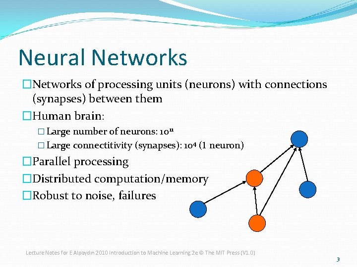
Neural Networks �Networks of processing units (neurons) with connections (synapses) between them �Human brain: � Large number of neurons: 1011 � Large connectitivity (synapses): 104 (1 neuron) �Parallel processing �Distributed computation/memory �Robust to noise, failures Lecture Notes for E Alpaydın 2010 Introduction to Machine Learning 2 e © The MIT Press (V 1. 0) 3

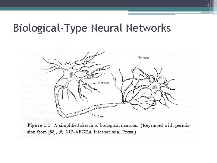
4 Biological-Type Neural Networks

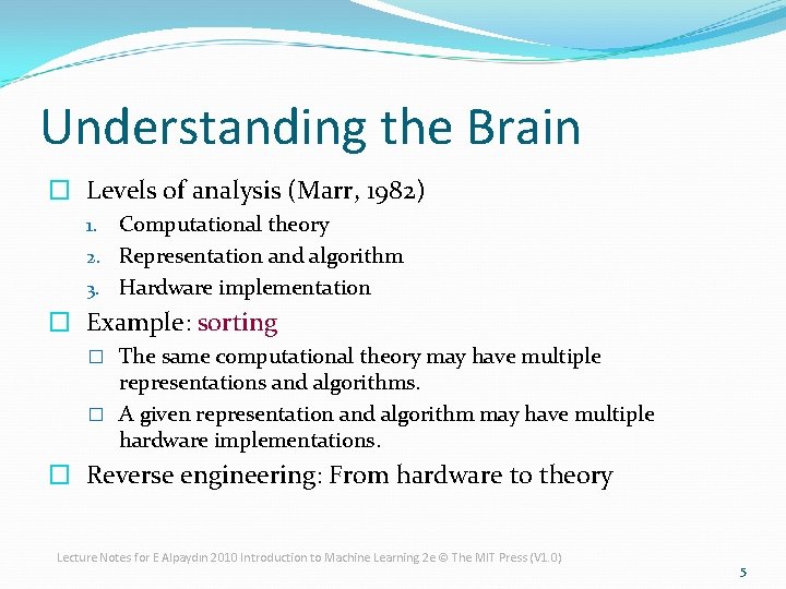
Understanding the Brain � Levels of analysis (Marr, 1982) Computational theory 2. Representation and algorithm 3. Hardware implementation 1. � Example: sorting � The same computational theory may have multiple representations and algorithms. � A given representation and algorithm may have multiple hardware implementations. � Reverse engineering: From hardware to theory Lecture Notes for E Alpaydın 2010 Introduction to Machine Learning 2 e © The MIT Press (V 1. 0) 5

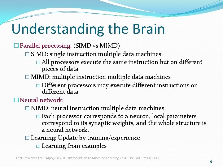
Understanding the Brain � Parallel processing: (SIMD vs MIMD) � SIMD: single instruction multiple data machines � All processors execute the same instruction but on different pieces of data � MIMD: multiple instruction multiple data machines � Different processors may execute different instructions on different data � Neural network: � NIMD: neural instruction multiple data machines � Each processor corresponds to a neuron, local parameters correspond to its synaptic weights, and the whole structure is a neural network. � Learning: Update by training/experience � Learning from examples Lecture Notes for E Alpaydın 2010 Introduction to Machine Learning 2 e © The MIT Press (V 1. 0) 6

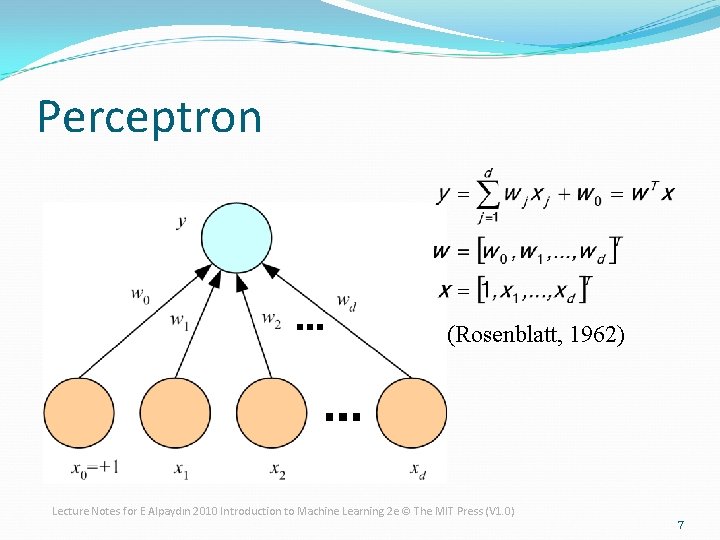
Perceptron (Rosenblatt, 1962) Lecture Notes for E Alpaydın 2010 Introduction to Machine Learning 2 e © The MIT Press (V 1. 0) 7

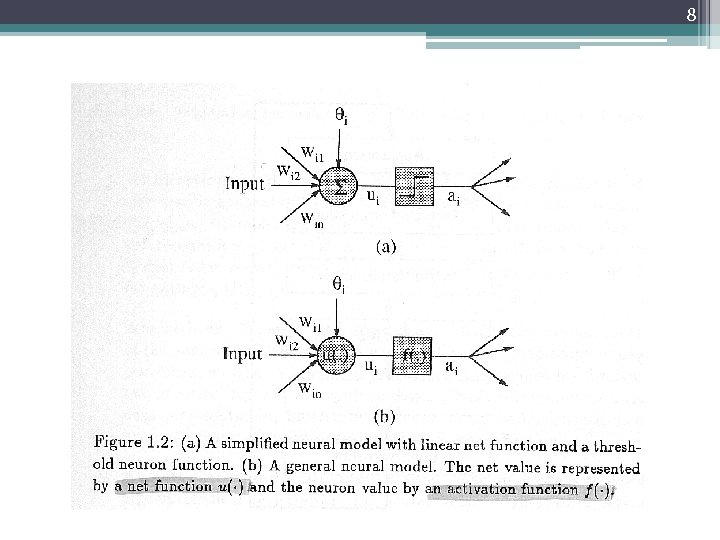
8

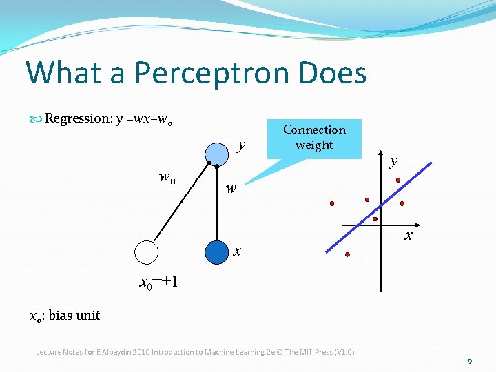
What a Perceptron Does Regression: y =wx+w 0 y w 0 Connection weight y w x x x 0=+1 x 0: bias unit Lecture Notes for E Alpaydın 2010 Introduction to Machine Learning 2 e © The MIT Press (V 1. 0) 9

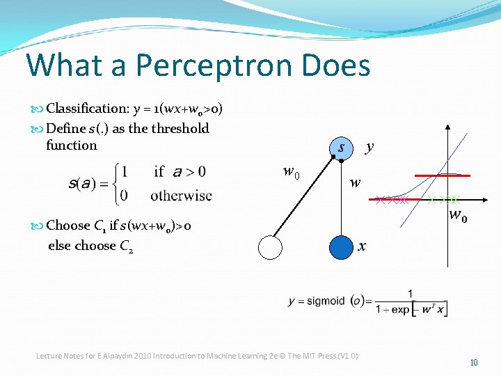
What a Perceptron Does Classification: y = 1(wx+w 0>0) Define s(. ) as the threshold function w 0 Choose C 1 if s(wx+w 0)>0 else choose C 2 y s w w 0 x Lecture Notes for E Alpaydın 2010 Introduction to Machine Learning 2 e © The MIT Press (V 1. 0) 10

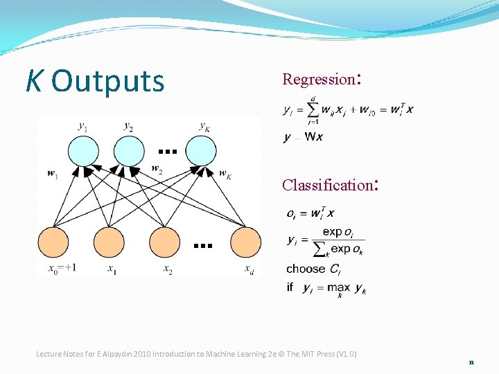
K Outputs Regression: Classification: Lecture Notes for E Alpaydın 2010 Introduction to Machine Learning 2 e © The MIT Press (V 1. 0) 11

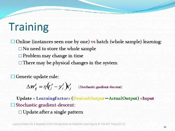
Training � Online (instances seen one by one) vs batch (whole sample) learning: � No need to store the whole sample � Problem may change in time � There may be physical changes in the system � Generic update rule: (Stochastic gradient-descent) Update = Learning. Factor× (Desired. Output－Actual. Output) ×Input � Stochastic gradient-descent: � Update after a single pattern Lecture Notes for E Alpaydın 2010 Introduction to Machine Learning 2 e © The MIT Press (V 1. 0) 12

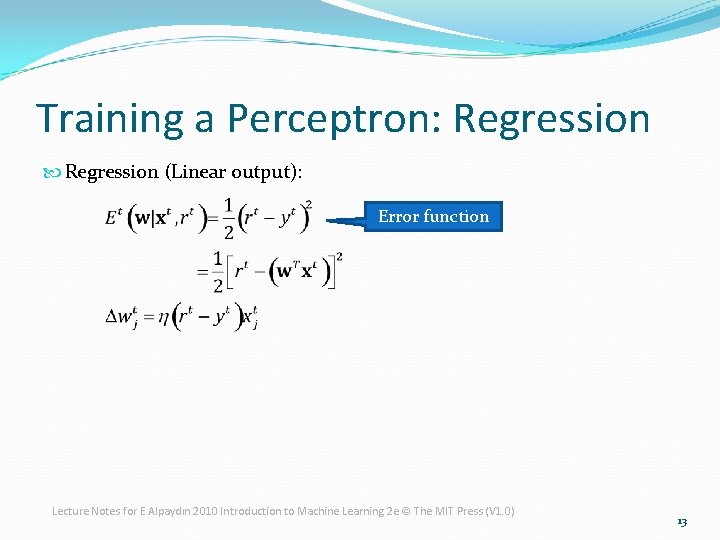
Training a Perceptron: Regression (Linear output): Error function Lecture Notes for E Alpaydın 2010 Introduction to Machine Learning 2 e © The MIT Press (V 1. 0) 13

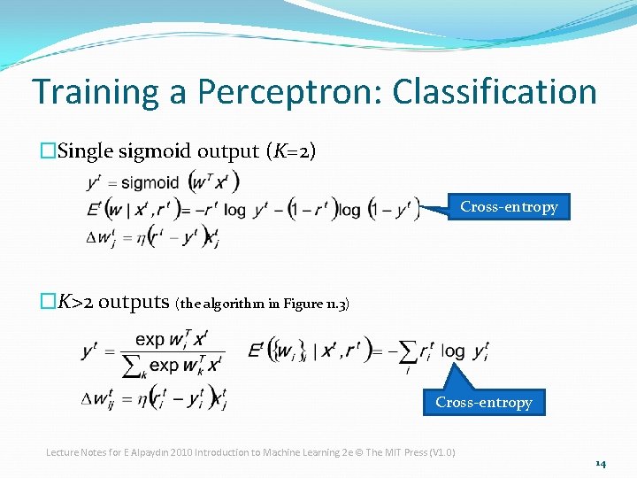
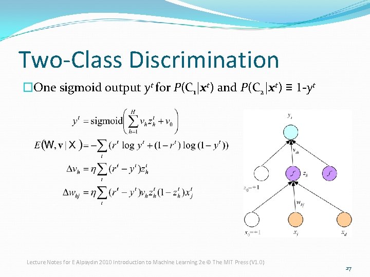
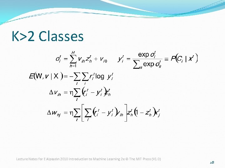
Training a Perceptron: Classification �Single sigmoid output (K=2) Cross-entropy �K>2 outputs (the algorithm in Figure 11. 3) Cross-entropy Lecture Notes for E Alpaydın 2010 Introduction to Machine Learning 2 e © The MIT Press (V 1. 0) 14

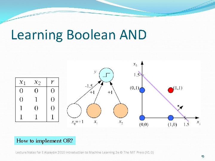
Learning Boolean AND How to implement OR? Lecture Notes for E Alpaydın 2010 Introduction to Machine Learning 2 e © The MIT Press (V 1. 0) 15

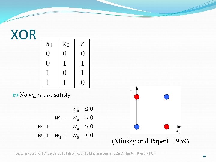
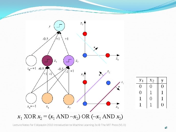
XOR No w 0, w 1, w 2 satisfy: (Minsky and Papert, 1969) Lecture Notes for E Alpaydın 2010 Introduction to Machine Learning 2 e © The MIT Press (V 1. 0) 16

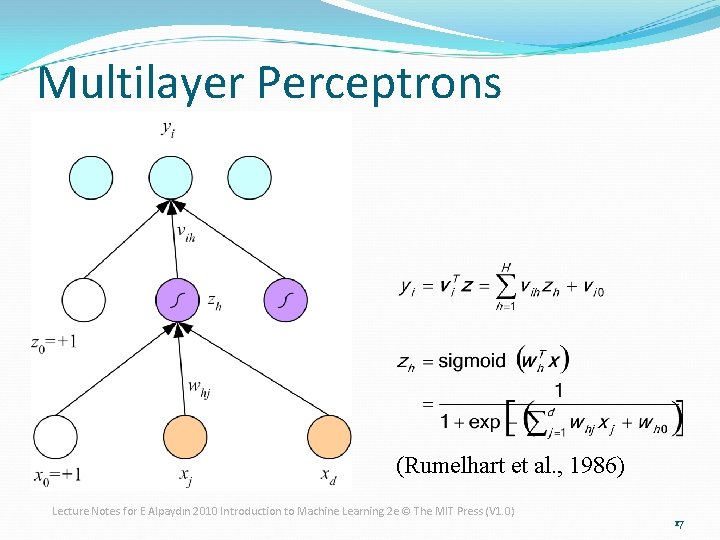
Multilayer Perceptrons (Rumelhart et al. , 1986) Lecture Notes for E Alpaydın 2010 Introduction to Machine Learning 2 e © The MIT Press (V 1. 0) 17

y x 1 XOR x 2 = (x 1 AND ~x 2) OR (~x 1 AND x 2) Lecture Notes for E Alpaydın 2010 Introduction to Machine Learning 2 e © The MIT Press (V 1. 0) 18

Hidden Layer � Do we have more hidden layers? � Yes! But complicate. � “Long and narrow” network vs “short and fat” network � Two hidden layers: (example) � For every input case of region, that region can be delimited by hyperplanes on all sides using hidden units on the first hidden layer. � A hidden unit in the second layer then ANDs them together to bound the region. � It has been proven that an MLP (Multilayer Perceptrons) with one hidden layer can learn any nonlinear function of the input. Lecture Notes for E Alpaydın 2010 Introduction to Machine Learning 2 e © The MIT Press (V 1. 0) 19

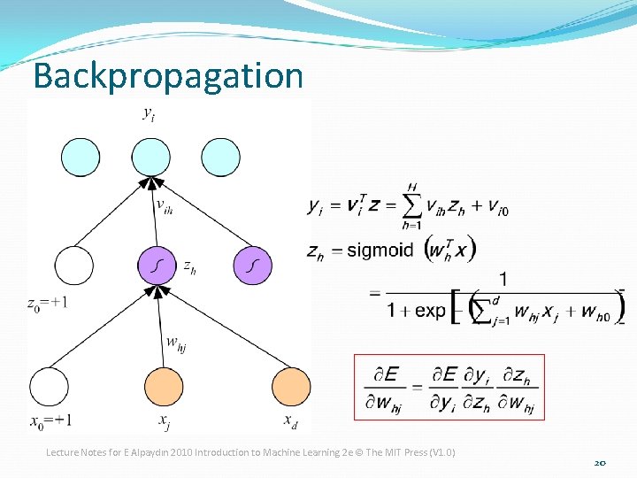
Backpropagation Lecture Notes for E Alpaydın 2010 Introduction to Machine Learning 2 e © The MIT Press (V 1. 0) 20

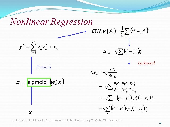
Nonlinear Regression Forward Backward x Lecture Notes for E Alpaydın 2010 Introduction to Machine Learning 2 e © The MIT Press (V 1. 0) 21

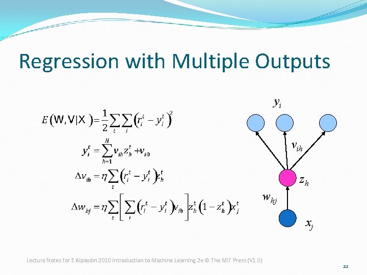
Regression with Multiple Outputs yi vih zh whj xj Lecture Notes for E Alpaydın 2010 Introduction to Machine Learning 2 e © The MIT Press (V 1. 0) 22

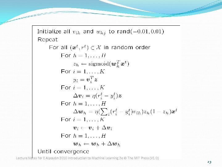
Lecture Notes for E Alpaydın 2010 Introduction to Machine Learning 2 e © The MIT Press (V 1. 0) 23

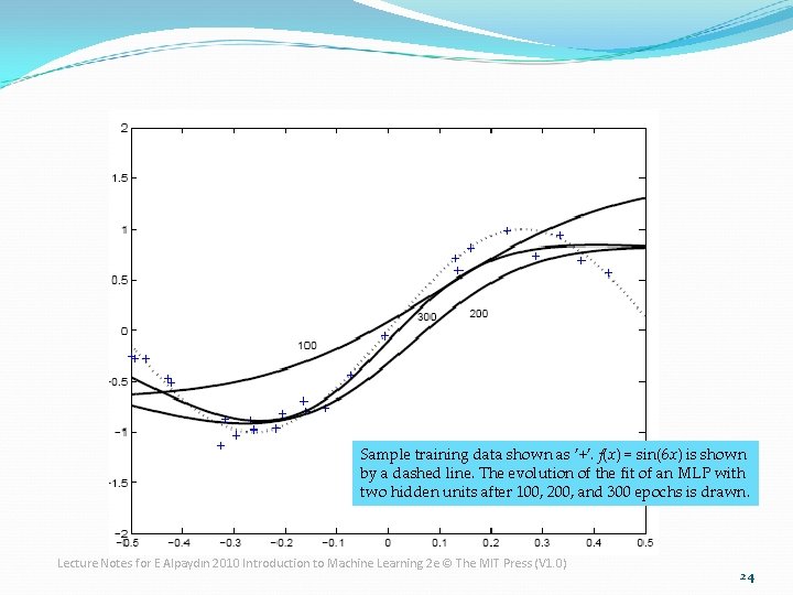
Sample training data shown as ’+’. f(x) = sin(6 x) is shown by a dashed line. The evolution of the fit of an MLP with two hidden units after 100, 200, and 300 epochs is drawn. Lecture Notes for E Alpaydın 2010 Introduction to Machine Learning 2 e © The MIT Press (V 1. 0) 24

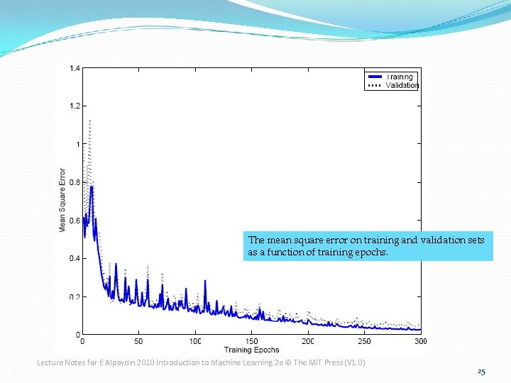
The mean square error on training and validation sets as a function of training epochs. Lecture Notes for E Alpaydın 2010 Introduction to Machine Learning 2 e © The MIT Press (V 1. 0) 25

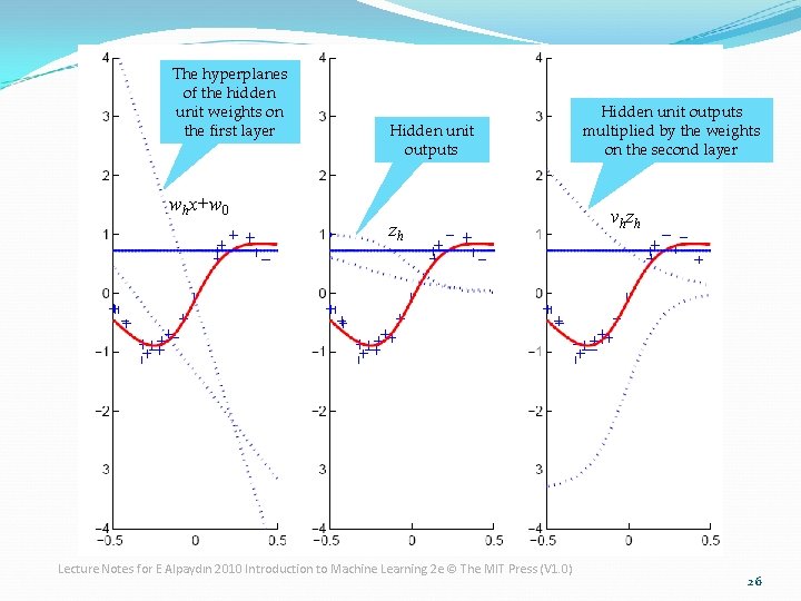
The hyperplanes of the hidden unit weights on the first layer whx+w 0 Hidden unit outputs zh Lecture Notes for E Alpaydın 2010 Introduction to Machine Learning 2 e © The MIT Press (V 1. 0) Hidden unit outputs multiplied by the weights on the second layer v h zh 26

Two-Class Discrimination �One sigmoid output yt for P(C 1|xt) and P(C 2|xt) ≡ 1 -yt Lecture Notes for E Alpaydın 2010 Introduction to Machine Learning 2 e © The MIT Press (V 1. 0) 27

K>2 Classes Lecture Notes for E Alpaydın 2010 Introduction to Machine Learning 2 e © The MIT Press (V 1. 0) 28

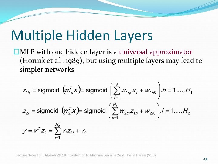
Multiple Hidden Layers �MLP with one hidden layer is a universal approximator (Hornik et al. , 1989), but using multiple layers may lead to simpler networks Lecture Notes for E Alpaydın 2010 Introduction to Machine Learning 2 e © The MIT Press (V 1. 0) 29

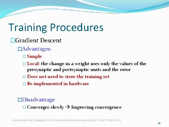
Training Procedures �Gradient Descent �Advantages: � Simple � Local: the change in a weight uses only the values of the presynaptic and postsynaptic units and the error � Does not need to store the training set � Be implemented in hardware �Disadvantage � Converges slowly Improving convergence Lecture Notes for E Alpaydın 2010 Introduction to Machine Learning 2 e © The MIT Press (V 1. 0) 30

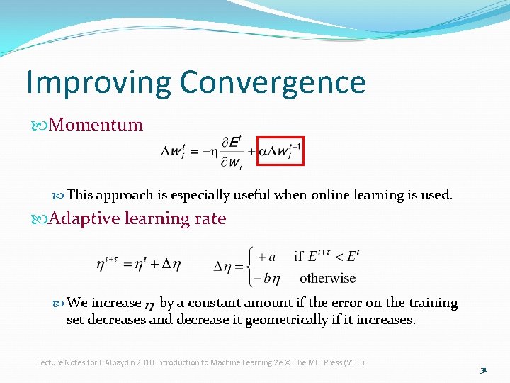
Improving Convergence Momentum This approach is especially useful when online learning is used. Adaptive learning rate We increase by a constant amount if the error on the training set decreases and decrease it geometrically if it increases. Lecture Notes for E Alpaydın 2010 Introduction to Machine Learning 2 e © The MIT Press (V 1. 0) 31

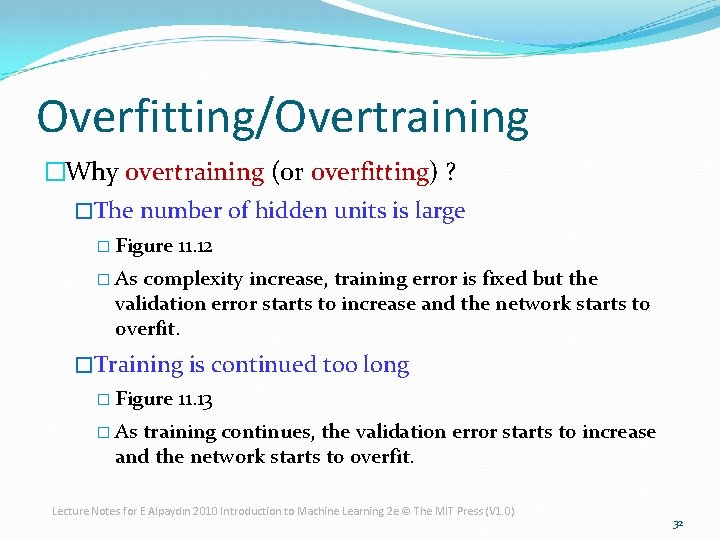
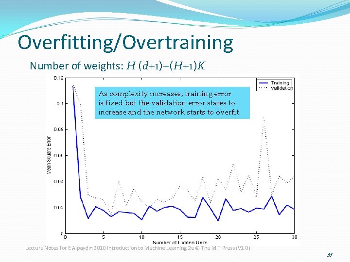
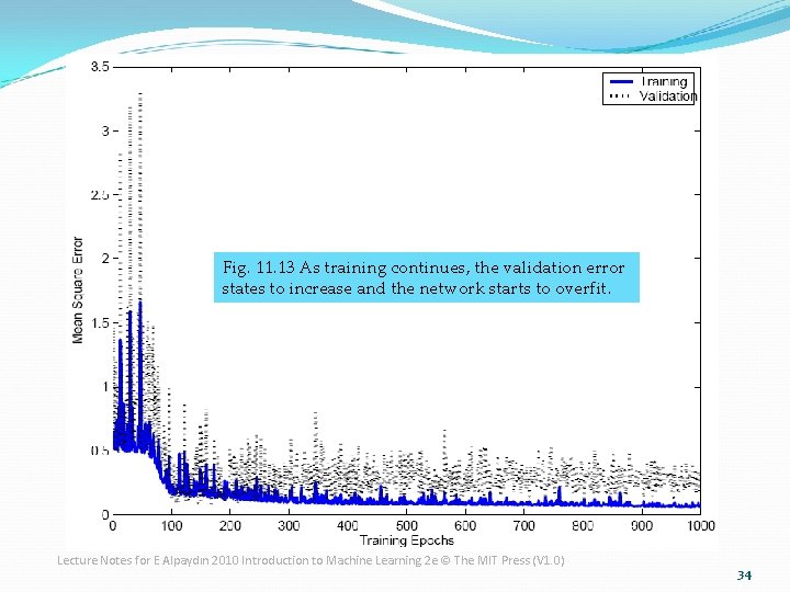
Overfitting/Overtraining �Why overtraining (or overfitting) ? �The number of hidden units is large � Figure 11. 12 � As complexity increase, training error is fixed but the validation error starts to increase and the network starts to overfit. �Training is continued too long � Figure 11. 13 � As training continues, the validation error starts to increase and the network starts to overfit. Lecture Notes for E Alpaydın 2010 Introduction to Machine Learning 2 e © The MIT Press (V 1. 0) 32

Overfitting/Overtraining Number of weights: H (d+1)+(H+1)K As complexity increases, training error is fixed but the validation error states to increase and the network starts to overfit. Lecture Notes for E Alpaydın 2010 Introduction to Machine Learning 2 e © The MIT Press (V 1. 0) 33

Fig. 11. 13 As training continues, the validation error states to increase and the network starts to overfit. Lecture Notes for E Alpaydın 2010 Introduction to Machine Learning 2 e © The MIT Press (V 1. 0) 34

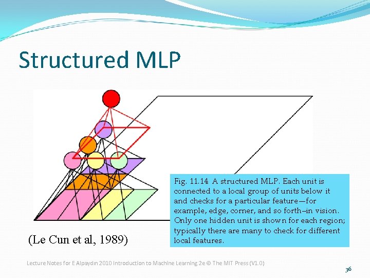
Structured MLP �How to reduce the number of connections? �Hierarchical cone: � If the input has a local structure, then when designing the MLP, hidden units are not connected to all input units because not all inputs are correlated. � For example: in vision recognition, detect local features like edges and corners � Figure 11. 14 � This decreased the number of connections and therefore the number of free parameters Lecture Notes for E Alpaydın 2010 Introduction to Machine Learning 2 e © The MIT Press (V 1. 0) 35

Structured MLP (Le Cun et al, 1989) Fig. 11. 14 A structured MLP. Each unit is connected to a local group of units below it and checks for a particular feature—for example, edge, corner, and so forth–in vision. Only one hidden unit is shown for each region; typically there are many to check for different local features. Lecture Notes for E Alpaydın 2010 Introduction to Machine Learning 2 e © The MIT Press (V 1. 0) 36

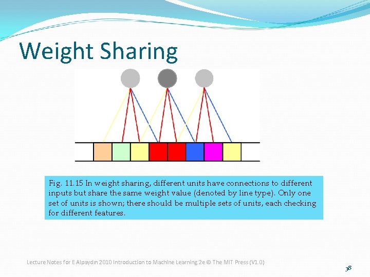
Structured MLP �How to reduce the number of connections? �Weight sharing: � In weight sharing, different units have connections to different inputs but share the same weight value. � Figure 11. 15: Only one set of units is shown; there should be multiple sets of units, each checking for different features. � For example: in visual recognition, detect features like oriented edges Lecture Notes for E Alpaydın 2010 Introduction to Machine Learning 2 e © The MIT Press (V 1. 0) 37

Weight Sharing Fig. 11. 15 In weight sharing, different units have connections to different inputs but share the same weight value (denoted by line type). Only one set of units is shown; there should be multiple sets of units, each checking for different features. Lecture Notes for E Alpaydın 2010 Introduction to Machine Learning 2 e © The MIT Press (V 1. 0) 38

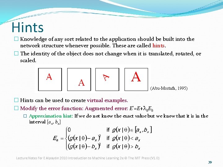
Hints � Knowledge of any sort related to the application should be built into the network structure whenever possible. These are called hints. � The identity of the object does not change when it is translated, rotated, or scaled. (Abu-Mostafa, 1995) � Hints can be used to create virtual examples. � Modify the error function: Augmented error: E’=E+λh. Eh � Approximation hint: If we do not know the exact value but we know that it is in the interval [ax, bx] Lecture Notes for E Alpaydın 2010 Introduction to Machine Learning 2 e © The MIT Press (V 1. 0) 39

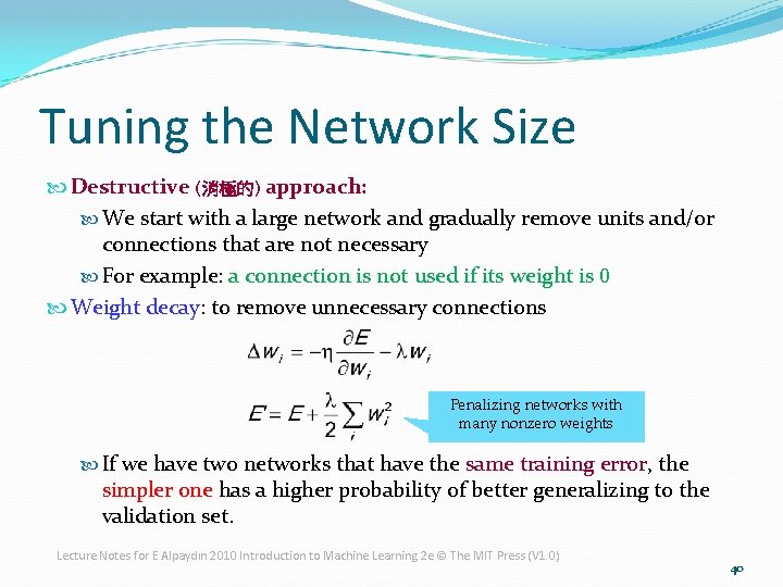
Tuning the Network Size Destructive (消極的) approach: We start with a large network and gradually remove units and/or connections that are not necessary For example: a connection is not used if its weight is 0 Weight decay: to remove unnecessary connections Penalizing networks with many nonzero weights If we have two networks that have the same training error, the simpler one has a higher probability of better generalizing to the validation set. Lecture Notes for E Alpaydın 2010 Introduction to Machine Learning 2 e © The MIT Press (V 1. 0) 40

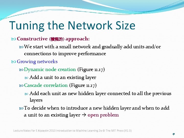
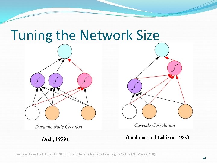
Tuning the Network Size Constructive (積極的) approach: We start with a small network and gradually add units and/or connections to improve performance Growing networks Dynamic node creation (Figure 11. 17) Add a unit to an existing layer Cascade correlation (Figure 11. 17) Add each unit as new hidden layer connected to all the previous layers To decide when to introduce a new hidden layer and when to add a unit to an existing layer open problem Lecture Notes for E Alpaydın 2010 Introduction to Machine Learning 2 e © The MIT Press (V 1. 0) 41

Tuning the Network Size (Ash, 1989) (Fahlman and Lebiere, 1989) Lecture Notes for E Alpaydın 2010 Introduction to Machine Learning 2 e © The MIT Press (V 1. 0) 42

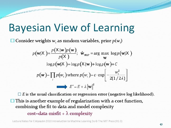
Bayesian View of Learning � Consider weights wi as random variables, prior p(wi) � E is the usual classification or regression error (negative log likelihood). � This is another example of regularization with a cost function, combining the fit to data and model complexity cost=data-misfit + λ complexity Lecture Notes for E Alpaydın 2010 Introduction to Machine Learning 2 e © The MIT Press (V 1. 0) 43

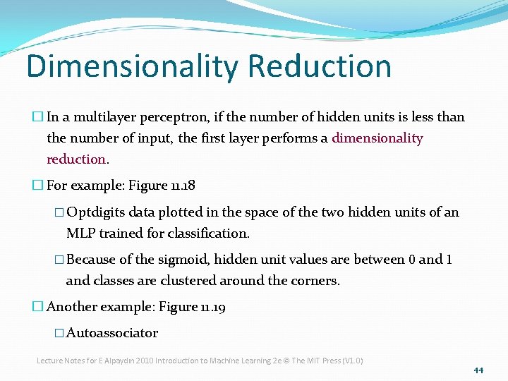
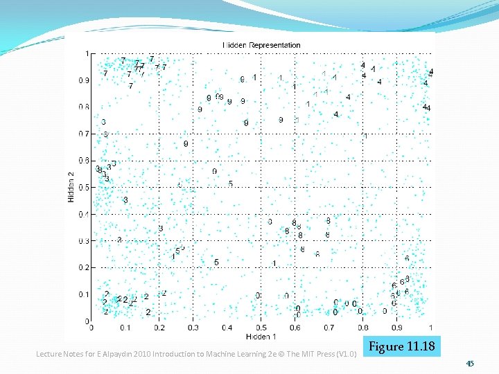
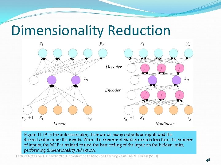
Dimensionality Reduction � In a multilayer perceptron, if the number of hidden units is less than the number of input, the first layer performs a dimensionality reduction. � For example: Figure 11. 18 � Optdigits data plotted in the space of the two hidden units of an MLP trained for classification. � Because of the sigmoid, hidden unit values are between 0 and 1 and classes are clustered around the corners. � Another example: Figure 11. 19 � Autoassociator Lecture Notes for E Alpaydın 2010 Introduction to Machine Learning 2 e © The MIT Press (V 1. 0) 44

Lecture Notes for E Alpaydın 2010 Introduction to Machine Learning 2 e © The MIT Press (V 1. 0) Figure 11. 18 45

Dimensionality Reduction Figure 11. 19 In the autoassociator, there as many outputs as inputs and the desired outputs are the inputs. When the number of hidden units is less than the number of inputs, the MLP is trained to find the best coding of the input on the hidden units, performing dimensionality reduction. Lecture Notes for E Alpaydın 2010 Introduction to Machine Learning 2 e © The MIT Press (V 1. 0) 46

Learning Time � In some applications, the input is temporal where we need to learn a temporal sequences. The output may change in time. � Examples: � Sequence recognition: Speech recognition � Sequence reproduction: Time-series prediction � Temporal association � Network architectures � Time-delay networks (Waibel et al. , 1989) � Recurrent networks (Rumelhart et al. , 1986) Lecture Notes for E Alpaydın 2010 Introduction to Machine Learning 2 e © The MIT Press (V 1. 0) 47

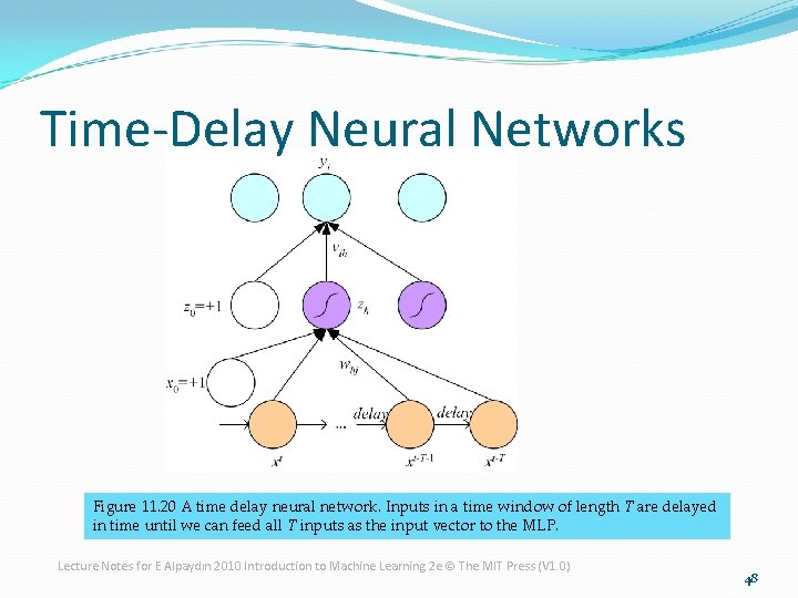
Time-Delay Neural Networks Figure 11. 20 A time delay neural network. Inputs in a time window of length T are delayed in time until we can feed all T inputs as the input vector to the MLP. Lecture Notes for E Alpaydın 2010 Introduction to Machine Learning 2 e © The MIT Press (V 1. 0) 48

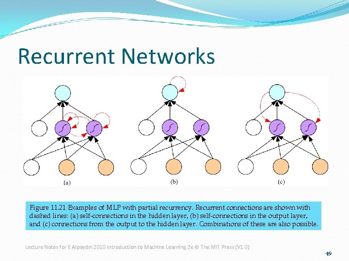
Recurrent Networks Figure 11. 21 Examples of MLP with partial recurrency. Recurrent connections are shown with dashed lines: (a) self-connections in the hidden layer, (b) self-connections in the output layer, and (c) connections from the output to the hidden layer. Combinations of these are also possible. Lecture Notes for E Alpaydın 2010 Introduction to Machine Learning 2 e © The MIT Press (V 1. 0) 49

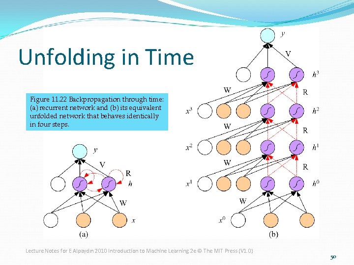
Unfolding in Time Figure 11. 22 Backpropagation through time: (a) recurrent network and (b) its equivalent unfolded network that behaves identically in four steps. Lecture Notes for E Alpaydın 2010 Introduction to Machine Learning 2 e © The MIT Press (V 1. 0) 50