Lecture on Correlation and Regression Analyses REVIEW Variable

Lecture on Correlation and Regression Analyses

REVIEW - Variable A variable is a characteristic that changes or varies over time or different individuals or objects under consideration. n. Broad Classification of Variables: n QUANTITATIVE n n DISCRETE CONTINUOUS QUALITATIVE

Types of Variable Qualitative n assumes values that are not numerical but can be categorized n categories may be identified by either nonnumerical descriptions or by numeric codes

Types of Variable Quantitative n indicates the quantity or amount of a characteristic n data are always numeric n can be discrete or continuous

Types of Quantitative Variables Discrete – variable with a finite or countable number of possible values Continuous – variable that assumes any value in a given interval 2. A. 5

Levels/Scales of Measurement Data may be classified into four hierarchical levels of measurement: Nominal Ordinal Interval Ratio Note: The type of statistical analysis that is appropriate for a particular variable depends on its level of measurement.

NOMINAL SCALE n n n Data collected are labels, names or categories. Frequencies or counts of observations belonging to the same category can be obtained. It is the lowest level of measurement.

ORDINAL SCALE n n Data collected are labels with implied ordering. The difference between two data labels is meaningless.

INTERVAL SCALE n n n Data can be ordered or ranked. The difference between two data values is meaningful. Data at this level may lack an absolute zero point.

RATIO SCALE Data have all the properties of the interval scale. n The number zero indicates the absence of the characteristic being measured. n It is the highest level of measurement. n

Learning Points – PART II 1. 2. 3. 4. 5. What is a correlation analysis What is a regression analysis When do we use correlation analysis? When do we use regression analysis? How do we compare regression versus correlation analysis?

CORRELATION ANALYSIS It is a statistical technique used to determine the strength of the relationship between two variables, X and Y. It provides a measure of strength of the linear relationship between two variables measured in at least interval scale. 5. F. 12

ILLUSTRATION The UP Admissions office may be interested in the relationship between UPCAT scores in Math and Reading Comprehension of UPCAT qualifiers. 5. F. 13

ILLUSTRATION A social scientist might be concerned with how a city’s crime rate is related to its unemployment rate. 5. F. 14

ILLUSTRATION A nutritionist might try to relate the quantity of carbohydrates in the diet consumed to the amount of sugar in the blood of diabetic individuals. 5. F. 15

PEARSON’S CORRELATION COEFFICIENT, where s. XY = covariance between X and Y s. X = standard deviation of the X values s. Y = standard deviation of the Y values N = number of paired observations in the population 5. F. 16
 together, >0")
PEARSON’S CORRELATION COEFFICIENT, Y as X Y X and Y increases (decreases) together, >0 X 5. F. 17
 while Y decreases (increases), < 0 Y as")
PEARSON’S CORRELATION COEFFICIENT, X increases (decreases) while Y decreases (increases), < 0 Y as X Y X 5. F. 18

PEARSON’S CORRELATION COEFFICIENT, No pattern Y X and Y have no linear relationship, = 0 X 5. F. 19

SAMPLE CORRELATION COEFFICIENT, r where s. XY s. X s. Y n = sample covariance of X and Y values = sample standard deviation of X values = sample standard deviation of Y values = sample size 5. F. 20

QUALITATIVE INTERPRETATION OF AND r Absolute Value of the Correlation Coefficient Strength of Linear Relationship 0. 0 – 0. 2 Very weak 0. 2 – 0. 4 Weak 0. 4 – 0. 6 Moderate 0. 6 – 0. 8 Strong 0. 8 – 1. 0 Very Strong 5. F. 21

EXAMPLE It is of interest to study the relationship between the number of hours spent studying and the student’s grade in an examination. A random sample of twenty students is selected and the data are given in the following table. Compute and interpret the sample correlation coefficient.
 Student Hours Studied 1 2 3 4 5 6 7 8")
EXAMPLE Score (%) Student Hours Studied 1 2 3 4 5 6 7 8 9 10 3 5 2 3 4 3 4 71 90 83 70 93 50 70 90 76 80 Slide No. V. F. 15 Student Hours Studied Score (%) 11 12 13 14 15 16 17 18 19 20 4 3 1 0 3 1 1 2 3 1 80 60 63 49 80 61 63 50 60 65

SCATTER PLOT Examination Score 100 90 80 70 60 50 40 0 1 2 3 4 5 Number of Hours Spent Studying 6

5. F. 25

Sample Correlation Coefficient Interpretation: There is a strong positive linear relationship between the number of hours the student spent studying for the exam and exam score of students.

TEST OF HYPOTHESIS ABOUT Ho: = 0; There is no linear relationship between X and Y. vs. Ha: 0; There is a linear relationship between X and Y. or Ha: > 0; There is a positive linear relationship between X and Y. or Ha: < 0; There is a negative linear relationship between X and Y. 5. F. 27

TEST OF HYPOTHESIS ABOUT The standardized form of the test statistic is which follows the Student’s t distribution with n - 2 df when the null hypothesis is TRUE. This is commonly referred to as ttest for correlation coefficient. 5. F. 28

TEST OF HYPOTHESIS ABOUT With a given level of significance, Alternative Hypothesis Ha: ≠ 0 (two-tailed test) Ha: >0 (one-tailed test) Ha: <0 (one-tailed test) 5. F. 29 Decision Rule Reject Ho if |tc| > ttab= tα/2(n-2). Fail to reject Ho, otherwise. Reject Ho if tc > ttab= tα(n-2). Fail to reject Ho, otherwise. Reject Ho if tc < ttab= - tα(n-2). Fail to reject Ho, otherwise.

EXAMPLE In the study of the relationship between the number of hours spent studying and the student’s grade in an examination. Is there evidence to say that longer number of hours spent studying is associated with higher exam scores at 5% level of significance?

Test of Hypothesis Ho: = 0; There is no linear relationship between the number of hours a student spent studying for the exam and his exam score. Ha: > 0; There is a positive linear relationship between the number of hours a student spent studying for the exam and his exam score.

Test of Hypothesis The test statistic is Test procedure: One-tailed t-test for correlation coefficient Decision rule: Reject Ho if tc > t. tab = t. 05(18) = 1. 734. Reject Ho, otherwise.

Test of Hypothesis Decision: Reject Ho. Conclusion: At α=5%, there is evidence to say that longer number of hours spent studying is associated with higher exam scores.

WORD OF CAUTION Correlation is a measure of the strength of linear relationship between two variables, with no suggestion of “cause and effect” or causal relationship. A correlation coefficient equal to zero only indicates lack of linear relationship and does not discount the possibility that other forms of relationship may exist. 5. F. 34

REGRESSION ANALYSIS A statistical technique used to study the functional relationship between variables which allows predicting the value of one variable, say Y, given the value of another variable, say X 5. F. 35

REGRESSION ANALYSIS n Y – dependent variable ¡ n n 5. F. 36 A variable whose variation/value depends on that of another. X – independent variable - A variable whose variation/value does not depend on that of another.

ILLUSTRATION The relationship between the number of hours spent studying and the student’s exam score may be expressed in equation form. This equation may be used to predict the student’s exam score knowing the number of hours the student spent studying. 5. F. 37

ILLUSTRATION A child’s height is studied to see whether it is related to his father’s height such that some equation can be used to predict a child’s height given his father’s height. Sales of a product may be related to the corresponding advertising expenditures. 5. F. 38

SAMPLE REGRESSION MODEL where b 0 = estimated Y-intercept; the predicted value of Y when X = 0; b 1 = estimated slope of the line; measures the change in the predicted value of Y per unit change in X 5. F. 39

ESTIMATORS where = mean of the Y values = mean of the X values = estimated common variance of the Y’s 5. F. 40

EXAMPLE In the previous example, we may want to predict the examination score of a student given the number of hours he spent studying. Estimated regression line: Predicted exam score for Xi = 2. 5 is 69. 44 ~ 69
 Student Hours Studied 1 2 3 4 5 6 7 8")
EXAMPLE Score (%) Student Hours Studied 1 2 3 4 5 6 7 8 9 10 3 5 2 3 4 3 4 71 90 83 70 93 50 70 90 76 80 Slide No. V. F. 15 Student Hours Studied Score (%) 11 12 13 14 15 16 17 18 19 20 4 3 1 0 3 1 1 2 3 1 80 60 63 49 80 61 63 50 60 65

TEST OF HYPOTHESIS ABOUT 1 Ho: b 1 = Ha: b 1 or Ha: b 1 > or Ha: b 1 < 5. F. 43 where is the hypothesized value of b 1

TEST OF HYPOTHESIS ABOUT 1 The standardized form of the test statistic is where and it follows the Student’s t distribution with n -2 df when the null hypothesis is TRUE. This is commonly referred to as t-test for regression coefficient. 5. F. 44

TEST OF HYPOTHESIS ABOUT 1 With a given level of significance, Alternative Hypothesis Ha: b 1 ≠ (two-tailed test) Ha: b 1 > (one-tailed test) Ha: b 1 < (one-tailed test) 5. F. 45 Decision Rule Reject Ho if |tc| > ttab= tα/2(n-2). Fail to reject Ho, otherwise. Reject Ho if tc > ttab= tα(n-2). Fail to reject Ho, otherwise. Reject Ho if tc < ttab= -tα(n-2). Fail to reject Ho, otherwise.

EXAMPLE Using the previous example, test at = 5% if a student’s examination score will increase by at least 1 percent with an additional hour of study time. Ho: Ha: < > Test statistic: Test procedure: One-tailed t-test for regression coefficient
 =")
EXAMPLE Decision Rule: Reject Ho if tc > t. tab = -t. 05(18) = -1. 734 Otherwise, Fail to reject Ho, Computations:

EXAMPLE Decision: Since tc= 4. 0791 > t. tab= -1. 734, we reject Ho. Conclusion: At =5%, the student’s exam score will increase by at least 1 percent for an additional hour of study time.

TEST OF HYPOTHESIS ABOUT 0 Ho: b 0 = where is the hypothesized value of b 0 Ha: b 0 or Ha: b 0 > or Ha: b 0 < 5. F. 49

TEST OF HYPOTHESIS ABOUT 0 The standardized form of the test statistic is where and it follows the Student’s t distribution with n -2 df when the null hypothesis is TRUE. This is commonly referred to as t-test for regression constant. 5. F. 50

TEST OF HYPOTHESIS ABOUT 0 With a given level of significance, Alternative Hypothesis Ha: b 0 ≠ (two-tailed test) Ha: b 0 > (one-tailed test) Ha: b 0 < (one-tailed test) 5. F. 51 Decision Rule Reject Ho if |tc| > ttab= tα/2(n-2). Fail to reject Ho, otherwise. Reject Ho if tc > ttab= tα(n-2). Fail to reject Ho, otherwise. Reject Ho if tc < ttab= - tα(n-2). Fail to reject Ho, otherwise.

EXAMPLE At = 5%, test if the data indicate that the student will fail (a score less than 60) if he did not study. Ho: Ha: > Test statistic: Test procedure: One-tailed t-test for regression constant
 = -1. 734 otherwise,")
EXAMPLE Decision rule: Reject Ho if tc > t. 05(18) = -1. 734 otherwise, Fail to reject Ho Computations: 40 + 2. 0485

EXAMPLE Decision: Since tc= 2. 0485 > ttab= -1. 734, we reject Ho. Conclusion: At = 5%, the student will get a score less than 60 or the student will fail if he/she did not study for the examination.
 - proportion of the total")
ADEQUACY OF THE MODEL Coefficient of Determination (R 2) - proportion of the total variation in Y that is explained by X, usually expressed in percent 5. F. 55

EXAMPLE Interpretation: Around 55% of the total variation in examination scores is explained by the number of hours spent studying. The remaining 45% is explained by other variables not in the model, or by the fact that the relationship is not exactly linear.

SUMMARY 1. 2. 3. 4. Correlation analysis Regression analysis Application with computer output Interpretation

Regression analysis n is a causality relationship, where you can predict the value of one variable given the values of the other variable/s.

Correlation analysis n is a relationship between two variables but without the causality clause. Regression analysis in policy analysis is usually used to forecast certain events. For example, our trend line is an example of a regression analysis.

Illustrations: n Knowing the effect of TV spot advertising on the number of people visiting the Family Planning clinic would allow the population commission official to decide rationally whether or not to increase the amount to be spent on TV spot advertising. The officer would be able to predict how many people the commission would be able to attract to the Family Planning clinic if it increased the number of TV ads run. (See series p. 176)

n The relationship between two variables (in our example, the number of TV ad runes and the number of people visiting Family Planning clinic can be summarized by a line. This is called the regression line. This is the line that we will use to predict the value of one variable, given the other.

Formula of the regression line: Where: b = the slope of the line; a = the Y intercept or the value of Y when x=0; e = the error term.

Example: Relationship between TV ads and number of people visiting the family planning clinic: Municipalities Number of TV ads (X) Number of people visiting the clinic (Y) 1 7 42 2 5 32 3 1 10 4 8 40 5 10 61 6 2 8 7 6 35 8 7 39 9 8 48 10 9 51 11 5 30 12 7 45 13 8 41 14 2 7 15 6 37 16 5 33
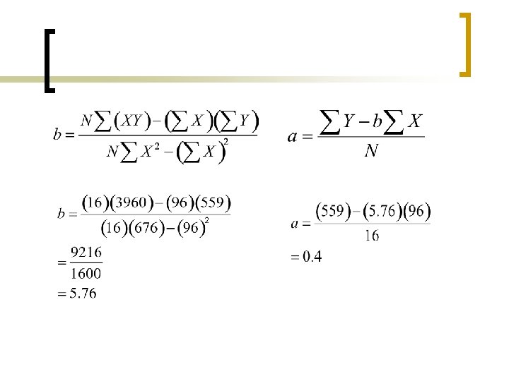

n The equation of the line is Y= 0. 4 + 5. 76 X n If X= 5, our predicted value for Y will be Y=. 4+ 5. 76 (5) = 29. 2 n If X=7, our predicted value for Y will be Y=. 4+ 5. 76 (7)= 40. 7 n Interpretation: An increase of one in the number of TV ad runs will generate a 5. 76 increase in the number of people visiting the family planning clinic. So the family planning officer can now proceed with evaluating the cost effectiveness of the program ads.

Coefficient of Determination n n The coefficient of determination is the percent variation in Y explained or accounted for by the variability of X. It is derived by squaring R and multiplying by 100. It is expressed in percentage term. Thus, if R=. 9, the coefficient of determination will be 81%. Formula:

Hypothesis Testing for a and bn We use the t-statistic to test the Hypothesis that a and b are significantly different from zero. n Excel analysis of the problem
, n-1")
Summary Output Revised Figure d. F: k, n-(k+1), n-1

DUMMY VARIABLE Represents nominal or categorical variable in the regression model For Example: Y= b 0 + b 1 X 1 + b 2 X 2 Y= scores, X 1=hours spent in studying, X 2=M/F taking a value of 1 if male, otherwise 0
- Slides: 69