Lecture Objectives SIMPLE vs Direct CFD solvers Advance

Lecture Objectives: SIMPLE vs. Direct CFD solvers Advance discretization methods Review

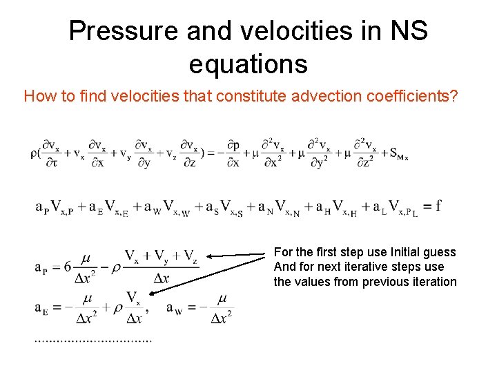
Pressure and velocities in NS equations How to find velocities that constitute advection coefficients? For the first step use Initial guess And for next iterative steps use the values from previous iteration

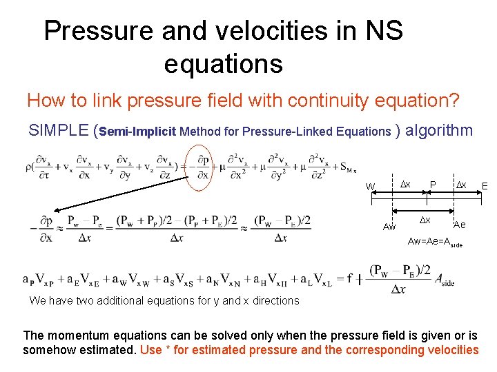
Pressure and velocities in NS equations How to link pressure field with continuity equation? SIMPLE (Semi-Implicit Method for Pressure-Linked Equations ) algorithm Dx W Aw P Dx Dx Ae Aw=Ae=Aside We have two additional equations for y and x directions The momentum equations can be solved only when the pressure field is given or is somehow estimated. Use * for estimated pressure and the corresponding velocities E

SIMPLE algorithm Guess pressure field: P*W, P*P, P*E, P*N , P*S, P*H, P*L 1) For this pressure field solve system of equations: x: y: z: ………………. . Solution is: 2) The pressure and velocity correction P = P* + P’ V = V* + V’ P’ – pressure correction V’ – velocity correction For all nodes E, W, N, S, … Substitute P=P* + P’ and V = V* + V’ into momentum equations and obtain V’=f(P’) V = V* + f(P’) 3) Substitute V = V* + f(P’) into continuity equation solve P’ and then V 4) Solve T , k , e equations

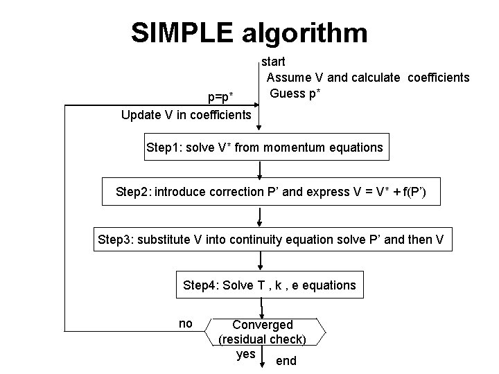
SIMPLE algorithm p=p* Update V in coefficients start Assume V and calculate coefficients Guess p* Step 1: solve V* from momentum equations Step 2: introduce correction P’ and express V = V* + f(P’) Step 3: substitute V into continuity equation solve P’ and then V Step 4: Solve T , k , e equations no Converged (residual check) yes end

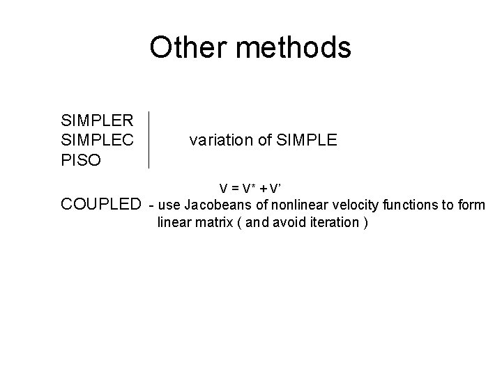
Other methods SIMPLER SIMPLEC PISO variation of SIMPLE V = V* + V’ COUPLED - use Jacobeans of nonlinear velocity functions to form linear matrix ( and avoid iteration )

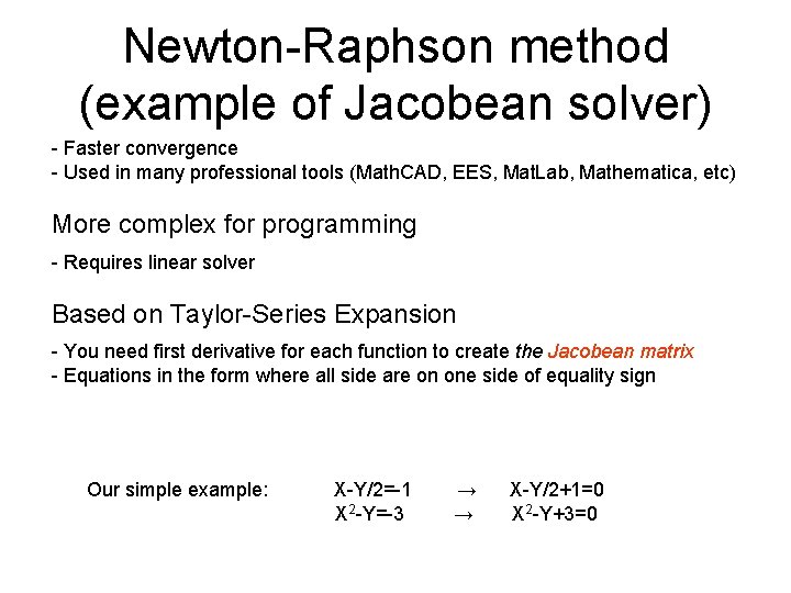
Newton-Raphson method (example of Jacobean solver) - Faster convergence - Used in many professional tools (Math. CAD, EES, Mat. Lab, Mathematica, etc) More complex for programming - Requires linear solver Based on Taylor-Series Expansion - You need first derivative for each function to create the Jacobean matrix - Equations in the form where all side are on one side of equality sign Our simple example: X-Y/2=-1 X 2 -Y=-3 → → X-Y/2+1=0 X 2 -Y+3=0

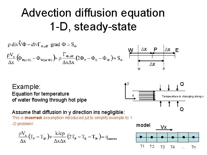
Advection diffusion equation 1 -D, steady-state Dx W w Example: P Dx Dx E e y Equation for temperature of water flowing through hot pipe Q x Temperature is changing along x Q Assume that diffusion in y direction ins negligible: This is incorrect assumption introduced jut to simplify example to 1 -D problem! model Vx T 1 T 3 T 2 T 4 … Tn

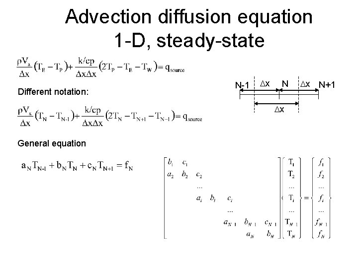
Advection diffusion equation 1 -D, steady-state Different notation: N-1 Dx N Dx General equation Dx N+1

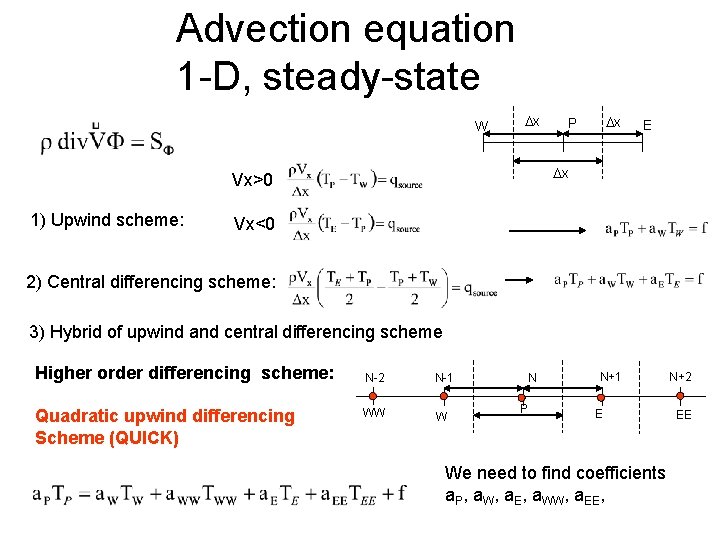
Advection equation 1 -D, steady-state W Dx E Dx Vx>0 1) Upwind scheme: Dx P Vx<0 2) Central differencing scheme: 3) Hybrid of upwind and central differencing scheme Higher order differencing scheme: Quadratic upwind differencing Scheme (QUICK) N-2 N-1 WW W N P N+1 E We need to find coefficients a. P, a. W, a. E, a. WW, a. EE, N+2 EE

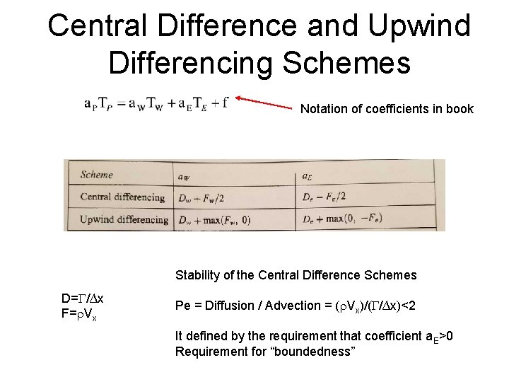
Central Difference and Upwind Differencing Schemes Notation of coefficients in book Stability of the Central Difference Schemes D= /∆x F= Vx Pe = Diffusion / Advection = ( Vx)/( /∆x)<2 It defined by the requirement that coefficient a. E>0 Requirement for “boundedness”

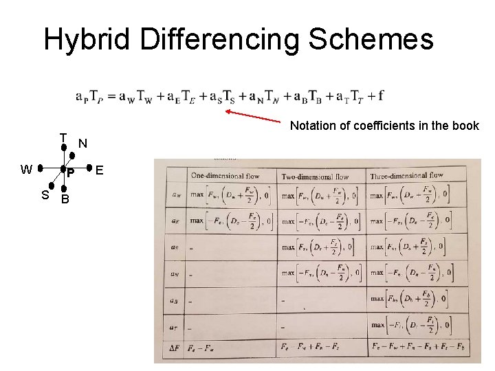
Hybrid Differencing Schemes Notation of coefficients in the book T N W P S B E

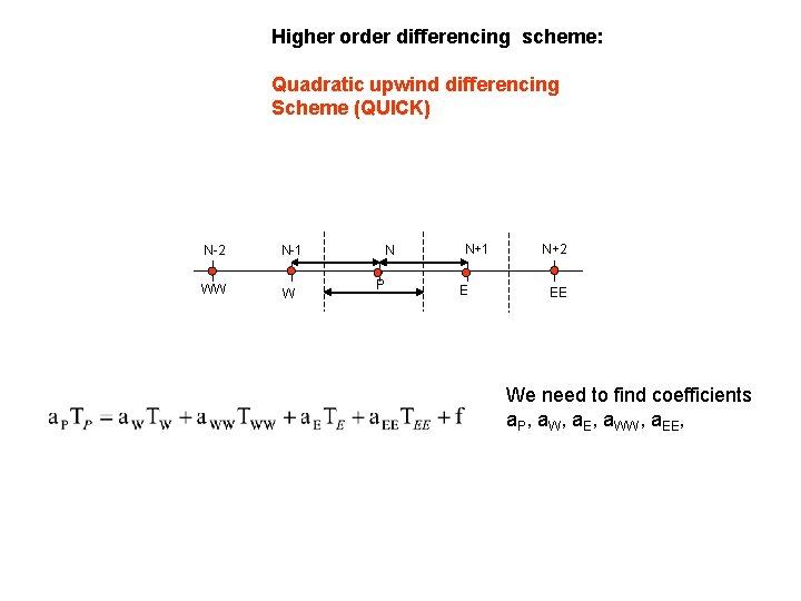
Higher order differencing scheme: Quadratic upwind differencing Scheme (QUICK) N-2 N-1 WW W N P N+1 E N+2 EE We need to find coefficients a. P, a. W, a. E, a. WW, a. EE,

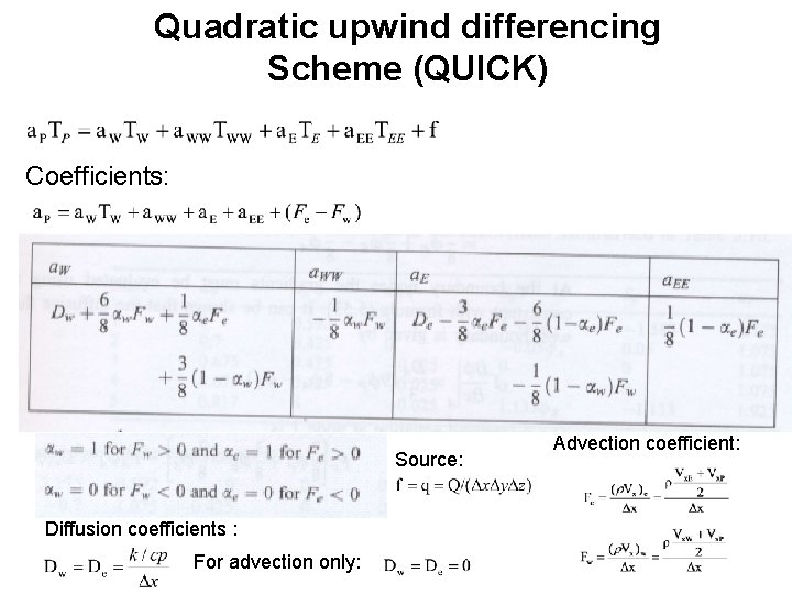
Quadratic upwind differencing Scheme (QUICK) Coefficients: Source: Diffusion coefficients : For advection only: Advection coefficient:

Course Review (so far)

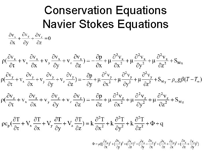
Conservation Equations Navier Stokes Equations

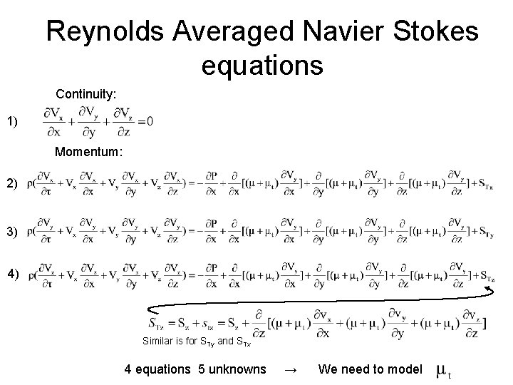
Reynolds Averaged Navier Stokes equations Continuity: 1) Momentum: 2) 3) 4) Similar is for STy and STx 4 equations 5 unknowns → We need to model

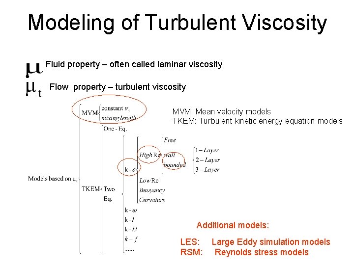
Modeling of Turbulent Viscosity Fluid property – often called laminar viscosity Flow property – turbulent viscosity MVM: Mean velocity models TKEM: Turbulent kinetic energy equation models Additional models: LES: RSM: Large Eddy simulation models Reynolds stress models

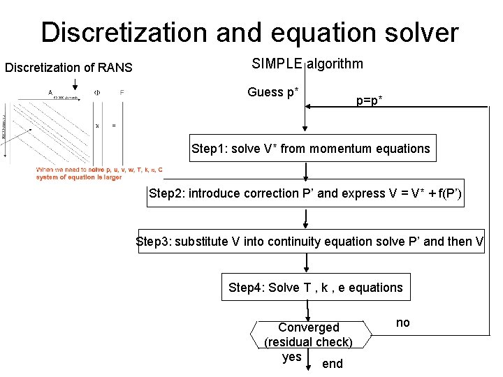
Discretization and equation solver Discretization of RANS SIMPLE algorithm Guess p* p=p* Step 1: solve V* from momentum equations Step 2: introduce correction P’ and express V = V* + f(P’) Step 3: substitute V into continuity equation solve P’ and then V Step 4: Solve T , k , e equations Converged (residual check) yes end no

CFD Software Airpak & Fluent Star. CCM+