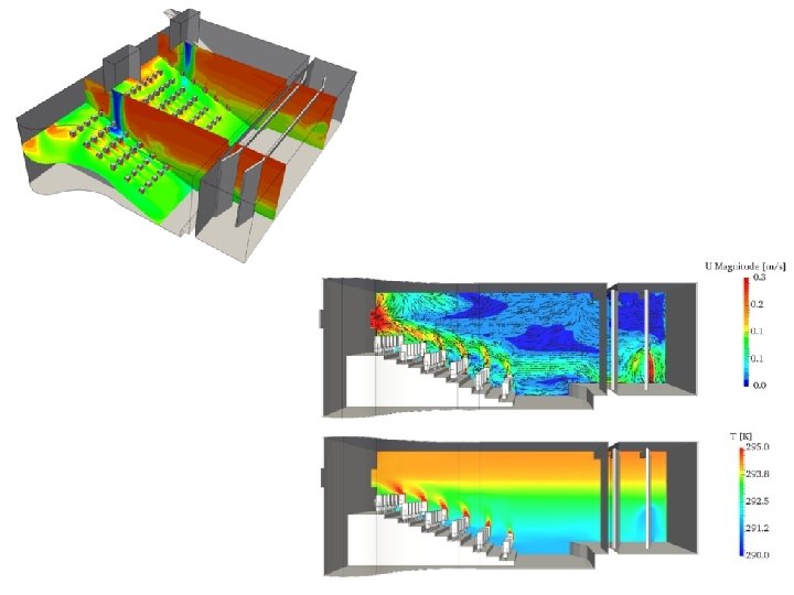
Lecture Objectives Discuss CFD results representation ventilation and

Lecture Objectives • Discuss CFD results representation – ventilation and contaminant removal effectiveness thermal comfort, and other • Review surface radiation models • Start with particle dynamics modeling • Learn more about LES

Air and Species Dispersion parameters Number of ACH quantitative indicator ACH - for total air - for fresh air Ventilation effectiveness qualitative indicator takes into account air distribution in the space Exposure qualitative indicator takes into account air distribution and source position and intensity

Indices - Age-of-air air-change effectiveness (EV) - Specific Contaminant Concentration contaminant removal effectiveness e

Single value IAQ indicators Ev and ε 1. Contaminant removal effectiveness (e) concentration at exhaust average contaminant concentration Contamination level 2. Air-change efficiency (Ev) shortest time for replacing the air average of local values of age of air Air freshness

Air-change efficiency (Ev) • Depends only on airflow pattern in a room • We need to calculate age of air ( ) Average time of exchange • What is the age of air at the exhaust? Type of flow – Perfect mixing – Piston (unidirectional) flow – Flow with stagnation and short-circuiting flow

Air exchange efficiency for characteristic room ventilation flow types Flow pattern Air-change Comparison with average efficiency time of exchange Unidirectional flow Perfect mixing 1 -2 1 n < exc < 2 n exc = n Short Circuiting 0 -1 exc > n

Contaminant removal effectiveness (e) • Depends on: - position of a contaminant source - Airflow in the room • Questions 1) Is the concentration of pollutant in the room with stratified flow larger or smaller that the concentration with perfect mixing? 2) How to find the concentration at exhaust of the room?

Differences and similarities of Ev and e Depending on the source position: - similar or - completely different air quality Ev = 0. 41 e = 0. 19 e = 2. 20

Thermal comfort Temperature and relative humidity

Thermal comfort Velocity Can create draft Draft is related to air temperature, air velocity, and turbulence intensity.

Thermal comfort Mean radiant temperature potential problems Asymmetry Warm ceiling (----) Cool wall (---) Cool ceiling (--) Warm wall (-)

Prediction of thermal comfort Predicted Mean Vote (PMV) PMV = +3 +2 +1 0 -1 -2 -3 hot warm slightly warm neutral slightly cool cold PMV = [0. 303 exp ( -0. 036 M ) + 0. 028 ] L L - Thermal load on the body Empirical correlations Ole Fanger L = Internal heat production – heat loss to the actual environment L = M - W - [( C sk + Rsk + Esk ) + ( Cres + Eres )] Predicted Percentage Dissatisfied (PPD) PPD = 100 - 95 exp [ - (0. 03353 PMV 4 + 0. 2179 PMV 2)] Further Details: ANSI/ASHRAE standard 55, ISO standard 7730

Surface Radiation Models Combined with CFD Example: Heat transfer through a window Cavity: CFD Domain

Multiphase flow can be classified in the following regimes: - gas-liquid or liquid-liquid flows - gas-solid flows – particle-laden flow: discrete solid particles in a continuous gas – pneumatic transport: flow pattern depends on factors such as solid loading, Reynolds numbers, and particle properties. Typical patterns are dune flow, slug flow, packed beds, and homogeneous flow. – fluidized beds: consist of a vertical cylinder containing particles where gas is introduced through a distributor. - liquid-solid flows - three-phase flows

Multiphase Flow Regimes Fluent user manual 2006

Boundary conditions for particle in the vicinity of surfaces Deposition velocity - ratio of the flux of particles at the considered surface and particle concentration per unit volume. For Nd particles deposited on a surface at time t, the deposition velocity is : Vde is the particle deposition velocity (m/s), N is the number of particles in air, A is the area of the considered surface (m²), V is the volume of the room (m 3). Resuspension Requires modeling based on empirical models or detail turbulence model (for example DNS) in boundary layer

Two basic approaches for modeling of particle dynamics • Lagrangian Model – particle tracking – For each particle ma=SF • Eulerian Model – Multiphase flow (fluid and particles) – Set of two systems of equations

Lagrangian Model particle tracking A trajectory of the particle in the vicinity of the spherical collector is governed by the Newton’s equation Forces that affect the particle m∙a=SF (r. Vvolume) particle ∙dvx/dt=SFx (r. Vvolume) particle ∙dvy/dt=SFy (r. Vvolume) particle ∙dvz/dt=SFz System of equation for each particle Solution is velocity and direction of each particle

Lagrangian Model particle tracking Basic equations - momentum equation based on Newton's second law Drag force due to the friction between particle and air - dp is the particle's diameter, - p is the particle density, - up and u are the particle and fluid instantaneous velocities in the i direction, - Fe represents the external forces (for example gravity force). This equation is solved at each time step for every particle. The particle position xi of each particle are obtained using the following equation: for each finite time step

Forces that affect the particle The drag force is the most significant force and it depends on Particle and fluid velocities Reynolds number defined for particle fluid velocity difference Drag coefficient: a 1, a 2, a 3 are constants that apply to smooth spherical particles or for non spherical particles: b 1, b 2, b 3, b 4 are constants that take into account non-spherical shape of particles

Forces that affect the particle External forces Electrostatic Thermophoretic Gravitation Brownian Lift force Brownian force – creates random movement of particles - for sub-micron particles, Lift force - lift due to shear Electrostatic – for charged particles Thermophoretic Force Small particles suspended in a gas that has a temperature gradient are exposed to a force in the direction opposite to that of the gradient. This phenomenon is known as thermophoresis.

Algorithm for CFD and particle tracking Unsteady state airflow Steady state airflow Airflow (u, v, w) for time step Steady state Injection of particles Particle distribution for time step + Airflow (u, v, w) for time step + Particle distribution for time step +2 Particle distribution for time step + …. . Case 1 when airflow is not affected by particle flow Case 2 particle dynamics affects the airflow One way coupling Two way coupling

Eulerian Model • Solve several sets of NS equations • Define the boundary conditions in-between phases Multiphase/Mixture Model • • Mixture model Secondary phase can be granular Applicable for solid-fluid simulations Granular physics Solve total granular pressure to momentum equation Use Solids viscosity for dispersed solid phase Density difference should be small. Useful mainly for liquid-solids multiphase systems There are models applicable for particles in the air

Multiphase flow can be classified in the following regimes: - gas-liquid or liquid-liquid flows - gas-solid flows – particle-laden flow: discrete solid particles in a continuous gas – pneumatic transport: flow pattern depends on factors such as solid loading, Reynolds numbers, and particle properties. Typical patterns are dune flow, slug flow, packed beds, and homogeneous flow. – fluidized beds: consist of a vertical cylinder containing particles where gas is introduced through a distributor. - liquid-solid flows - three-phase flows

Examples of LES: • • https: //www. youtube. com/watch? v=y. RSoil. RCu. Es https: //www. youtube. com/watch? v=y 1 s. SRXFBN 7 k https: //www. youtube. com/watch? v=d. We 3 fnfo 9 WQ https: //www. youtube. com/watch? v=e 1 Tbk. LIDWys https: //www. youtube. com/watch? v=i. JIRrk 7 t. Kws https: //www. youtube. com/watch? v=NClf. Gdfw. WTA https: //www. youtube. com/watch? v=hz 7 Uj. N_v. Yuw Vorticity formula:

LES vs RANS: LES: Low pass filter – resolve large scale eddies Model effect of small scale eddies Cut-off scale ∆ (space grid), cut of time scale ∆

LES Similar to RANS we are using effective viscosity for LES: Gradient of velocity tensor: is the rate-of-strain tensor for the resolved scale Finally: So no additional transport equation! This is Sub. Grid Scale (SGS) model Smagorinsky model (1963) eddy viscosity is model There are Many more: Algebraic Dynamic model Dynamic Global-Coefficient model Localized Dynamic model

LES • Time Step • Depends on the length scale and velocity – Courant–Friedrichs–Lewy (CFL) number • condition for convergence while solving hyperbolic differential equations

Multizone modeling CONTAM and COMIS • http: //www. bfrl. nist. gov/IAQanalysis/ • NO momentum equation • Just pressure, temperature, and continuity • Depends heavily on boundary condition and orifice coefficients that define flow between zones • Good for buoyancy driven flow

Boundary condition for multizone modeling • Exterior pressure (wind) • Temperature distribution (requires some assumption or energy modeling)

Wind pressure around building Very complex and unsteady For multizone we are introducing many simplifications: ….

Multizone vs. Moltizonla • “Multizonal” is like CFD (detailed grid with no orifice between i- between zones) but no momentum equation