Lecture Linear systems and convolution Linearity Conditions Let

Lecture: Linear systems and convolution

Linearity Conditions Let f 1(x, y) and f 2(x, y) describe two objects we want to image. f 1(x, y) can be any object and represent any characteristic of the object. (e. g. color, intensity, temperature, texture, X-ray absorption, etc. ) Assume each is imaged by some imaging device (system). Let f 1(x, y) → g 1(x, y) f 2(x, y) → g 2(x, y) Let’s scale each object and combine them to form a new object. a f 1(x, y) + b f 2(x, y) If the system is linear, output is a g 1(x, y) + b g 2(x, y)

Linearity Example: Is this a linear system?

Linearity Example: Is this a linear system? 9→ 3 16 → 4 9 + 16 = 25 → 5 3+4≠ 5 Not linear.

Example in medical imaging: Doubling the X-ray photons → doubles those transmitted Doubling the nuclear medicine → doubles the reception source energy MR: Maximum output voltage is 4 V. Now double the water: The A/D converter system is non-linear after 4 m. V. (overranging)

Linearity allows decomposition of functions Linearity allows us to decompose our input into smaller, elementary objects. Output is the sum of the system’s response to these basic objects.

Elementary Function: The two-dimensional delta function δ(x, y) has infinitesimal width and infinite amplitude. Key: δ(x, y) Volume under function is 1.

The delta function as a limit of another function Powerful to express δ(x, y) as the limit of a function Gaussian: lim a 2 exp[- a 2(x 2+y 2)] = δ(x, y) 2 D Rect Function: lim a 2 Π (ax) Π(ay) = δ(x, y) where Π(x) = 1 for |x| < ½ For this reason, δ(bx) = (1/|b|) δ(x)

Sifting property of the delta function The delta function at x 1 = ε, y 1= η has sifted out f (x 1, y 1) at that point. One can view f (x 1, y 1) as a collection of delta functions, each weighted by f (ε, η).

Imaging Analyzed with System Operators From previous page: Let system operator (imaging modality) be Why the new coordinate system (x 2, y 2)? , so that

Imaging Analyzed with System Operators Then, Generally blurred object System operating on entire input object f 1 (x 1, y 1) By linearity, we can consider the output as a sum of the outputs from all the weighted elementary delta functions. Then,

System response to a two-dimensional delta function Substituting this into yields the Superposition Integral

Example in medical imaging: Consider a nuclear study of a liver with a tumor point source at x 1 = ε, y 1= η Radiation is detected at the detector plane. To obtain a general result, we need to know all combinations h(x 2, y 2; ε, η ) By “general result”, we mean that we could calculate the image I(x 2, y 2) for any source input S(x 1, y 1)

Time invariance A system is time invariant if its output depends only on relative time of the input, not absolute time. To test if this quality exists for a system, delay the input by t 0. If the output shifts by the same amount, the system is time invariant i. e. f(t) → f(t - to) → input delay g(t) g(t - to) output delay Is f(t) → f(at) → g(t) (an audio compressor) time invariant?

Time invariance A system is time invariant if its output depends only on relative time of the input, not absolute time. To test if this quality exists for a system, delay the input by t 0. If the output shifts by the same amount, the system is time invariant i. e. f(t) → f(t - to) → input delay g(t) g(t - to) output delay Is f(t) → f(at) → g(t) (an audio compressor) time invariant? f(t - to) → f(at) → f(a(t – to)) - output of audio compressor f(at – to) - shifted version of output (this would be a time invariant system. ) So f(t) → f(at) = g(t) is not time invariant.

Space or shift invariance A system is space (or shift) invariant if its output depends only on relative position of the input, not absolute position. If you shift input in the plane, → The response shifts, but the shape of the response stays the same. If the system is shift invariant, h(x 2, y 2; ε, η ) = h(x 2 -ε , y 2 -η ) and the superposition integral becomes the 2 D convolution function: Notation: g = f**h (** sometimes implies two-dimensional convolution, as opposed to g = f*h for one dimension. Often we will use * with 2 D and 3 D functions and imply 2 D or 3 D convolution. )

One-dimensional convolution example: g(x) = Π(x)*Π(x/2) Recall: Π(x) = 1 for |x| < ½ Π(x/2) = 1 for |x|/2 < ½ or |x| < 1 Flip one object and drag across the other. flip delay

One-dimensional convolution example, continued: Case 1: no overlap of Π(x-x’) and Π(x’/2) Case 2: partial overlap of Π(x-x’) and Π(x’/2)

One-dimensional convolution example, continued(2): Case 3: complete overlap Case 4: partial overlap Case 5: no overlap

One-dimensional convolution example, continued(3): Result of convolution:

Two-dimensional convolution sliding of flipped object

2 D Convolution of a square with a rectangle.

2 D Convolution of letter E - 3 D plots

2 D Convolution of letter E - Grayscale images

Review of Fourier Transforms

1 -D Fourier Theory Fourier Transform: Inverse Fourier Transform: You may have seen the Fourier transform and its inverse written as: Why use the top version instead? 1) No scaling factor (1/2 ); easier to remember. 2) Easier to think in Hz than in radians/s

Review of 1 -D Fourier Theory, continued Let’s generalize so we can consider functions of variables other than time. Fourier Transform: Inverse Fourier Transform:

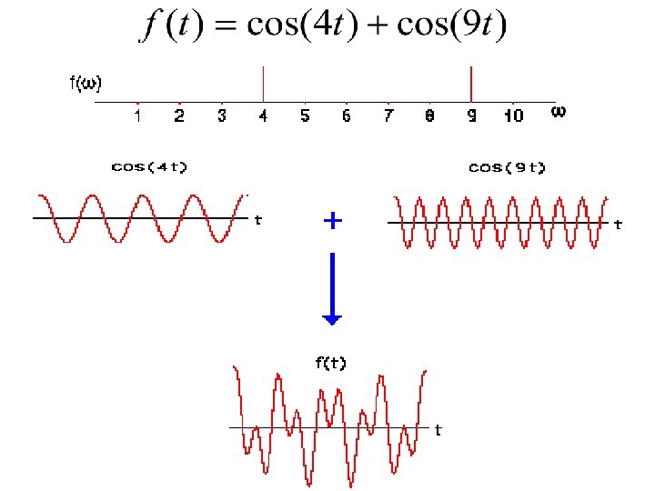
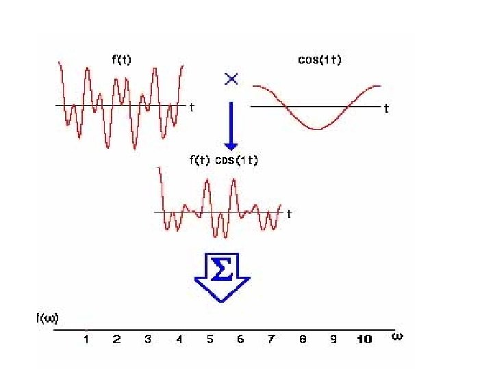
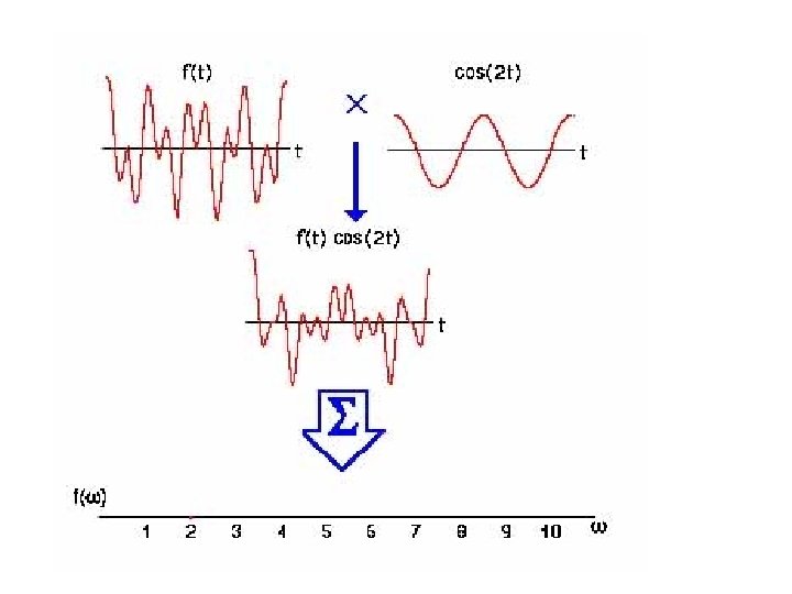
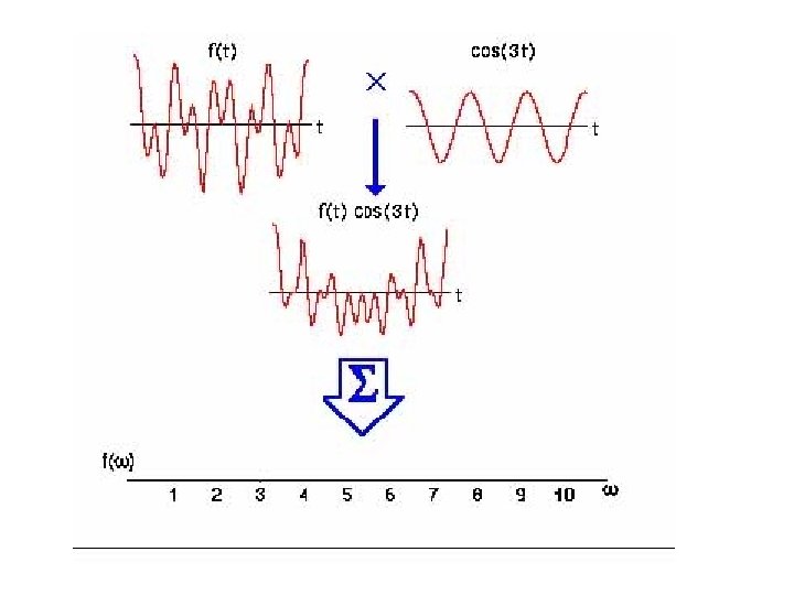
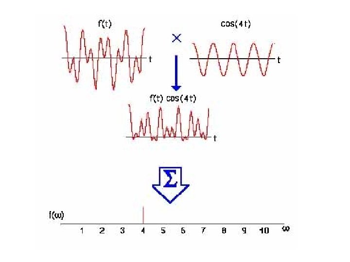
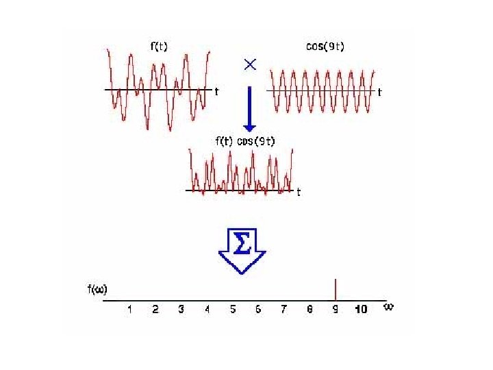
Review of 1 -D Fourier theory, continued (2) Orthogonal basis functions f(x) can be viewed as as a linear combination of the complex exponential basis functions. F(u) gives us the magnitude and phase of each of the exponentials that comprise f(x). In fact, the Fourier integral works by sifting out the portion of f(x) that is comprised of the function exp(+i 2π uo x).

Some Fourier Transform Pairs and Definitions -1/2 -1 1

MX (Real) MY (Imaginary)

MX (Real) MY (Imaginary)

Some Fourier Transform Pairs and Definitions, continued

1 -D Fourier transform properties If Linearity: f(x) ↔ F(u) and h(x) ↔ H(u) , af(x) + bh(x) ↔ a. F(u) + b. H(u) Scaling: f(ax) ↔ Shift: f(x-a) ↔

1 -D Fourier transform properties, continued. Say g(x) ↔ G(u). Then, Derivative Theorem: (Emphasizes higher frequencies – high pass filter) Integral Theorem: (Emphasizes lower frequencies – low pass filter)

Even and odd functions and Fourier transforms Any function g(x) can be uniquely decomposed into an even and odd function. e(x) = ½( g(x) + g(-x) ) o(x) = ½( g(x) – g(-x) ) For example, e 1 + e 2 = o 1 + o 2 = even odd e 1 · e 2 o 1 · o 2 e 1 · o 1 = = = even odd

Fourier transforms of even and odd functions Consider the Fourier transforms of even and odd functions. g(x) = e(x) + o(x) Sidebar: E(u) and O(u) can both be complex if e(x) and o(x) are complex. If g(x) is even, then G(u) is even. If g(x) is odd, then G(u) is odd.

Special Cases For a real-valued g(x) ( e(x) , o(x) are both real ), Real part is even in u Imaginary part is odd in u So, G(u) = G*(-u), which is the definition of Hermitian Symmetry: G(u) = G*(-u) (even in magnitude, odd in phase)

Example problem Find the Fourier transform of

Example problem: Answer. Find the Fourier transform of f(x) = Π(x /4) – Λ(x /2) +. 5Λ(x) Using the Fourier transforms of Π and Λ and the linearity and scaling properties, F(u) = 4 sinc(4 u) - 2 sinc 2(2 u) +. 5 sinc 2(u)

Example problem: Alternative Answer. Find the Fourier transform of f(x) = Π(x /4) – 0. 5((Π(x /3) * Π(x)) – 2 1 0 1 2 * – 1 -. 5 0. 5 1 Using the Fourier transforms of Π and Λ and the linearity and scaling and convolution properties , F(u) = 4 sinc(4 u) – 1. 5 sinc(3 u)sinc(u)

2 D Fourier Transfrom

Original 256 x 256 F(u, v) space

256 x 256 Image ( Interpolated by Powerpoin

Zero Padding x 2 ( 512 x 512 Recon, 256 x 256

Zero Padding x 2 ( 512 x 512 Recon of 256 x 256 F

Zero Padding x 4 ( 1024 x 1024 Recon, 256 x 256 F

Zero Padding x 4 ( 1024 x 1024 Recon of 256 x 256

FT Conventions - 1 D in Matlab 1 D Fourier Transform phase (L) >>l = z(33, : ); >>L = fft(l); abs (L) l 1 0 33 sample # x [Matlab] 64 1 xmax 0 33 sample # f. N/2 u 64 f. N

abs (L 2) 1 D FT - 2 xfftshift >>L 2 = fftshift(fft(l)); phase (L 2) Center Fourier Domain 1 33 sample # -f. N/2 0 u 64 (N-1)/N*f. N/2

fftshift in 2 D Use fftshift for 2 D functions >>smiley 2 = fftshift(smiley);

2 D Discrete Fourier Transform >>Z=fftshift(fft 2(z)); >>whos >>figure >>imshow(real(Z)) >>imshow(real(Z), []) >>colorbar Real (Z) >>figure >>imshow(imag(Z), []) >>colorbar Imag (Z)

2 D DFT - Zero Filling Interpolating Fourier space by zerofilling in image space >>z_zf = zeros(256); >>z_zf(97: 160, 97: 160) = z; >>Z_ZF = fftshift(fft 2(z_zf)); >>figure >>imshow(abs(Z_ZF), []) >>colorbar Magnitude (Z_ZF) >>figure >>imshow(angle(Z_ZF), []) >>colorbar Phase (Z_ZF)

2 D DFT - Voxel Shifts Shift image: 5 voxels up and 2 voxels left >>z_s = zeros(256); >>z_s(92: 155, 95: 158) = z; >>Z_S = fftshift(fft 2(z_s)); >>figure >>imshow(abs(Z_S), []) >>colorbar Magnitude (Z_S) >>figure >>imshow(angle(Z_S), [ ]) >>colorbar Phase (Z_S)