Lecture I Introduction to complex networks Santo Fortunato

Lecture I Introduction to complex networks Santo Fortunato

References Ü Evolution of networks S. N. Dorogovtsev, J. F. F. Mendes, Adv. Phys. 51, 1079 (2002), mat/0106144 cond- Ü Statistical mechanics of complex networks R. Albert, A-L Barabasi Reviews of Modern Physics 74, 47 (2002), mat/0106096 Ü The structure and function of complex networks M. E. J. Newman, SIAM Review 45, 167 -256 (2003), mat/0303516 cond- Ü Complex networks: structure and dynamics S. Ü Community detection in graphs S. Boccaletti, V. Latora, Y. Moreno, M. Chavez, D. -U. Hwang Physics Reports 424, 175 -308 (2006) Fortunato, Physics Reports 486, 75 -174 (2010) ar. Xiv: 0906. 0612

Plan of the course I. Networks: definitions, characteristics, basic concepts in graph theory II. Real world networks: basic properties III. Models IV. Community structure II VI. Dynamic processes in networks

What is a network? Network or graph=set of vertices joined by edges very abstract representation very general convenient to describe many different systems

Some examples Vertices Edges Social networks Individuals Social relations Internet Routers AS Cables Commercial agreements WWW Webpages Hyperlinks Protein interaction networks Proteins Chemical reactions and many more (email, P 2 P, foodwebs, transport…. )

Interdisciplinary science Science of complex networks: -graph theory -sociology -communication science -biology -physics -computer science

Interdisciplinary science Science of complex networks: Ü Empirics Ü Characterization Ü Modeling Ü Dynamical processes

Graph Theory Origin: Leonhard Euler (1736) L. Euler, Solutio problematis ad geometriam situs pertinentis, Comment. Academiae Sci. J. Petropolitanae 8, 128 -140 (1736)

Graph theory: basics Graph G=(V, E) Ü V=set of nodes/vertices i=1, …, n Ü E=set of links/edges (i, j), m i Bidirectional communication/ interaction j Undirected edge: i Directed edge: j

Graph theory: basics Maximum number of edges Ü Undirected: n(n-1)/2 Ü Directed: n(n-1) Complete graph: (all to all interaction/communication)

Adjacency matrix n vertices i=1, …, n 1 if (i, j) 0 if (i, j) aij= 0 1 2 3 0 0 1 1 1 0 1 1 2 1 1 0 1 E E 3 1 1 1 0 3 2

Adjacency matrix n vertices i=1, …, n 1 if (i, j) 0 if (i, j) aij= 0 1 2 3 0 0 1 1 2 0 1 E E 3 0 1 1 0 Symmetric for undirected networks 0 3 1 2

Adjacency matrix n vertices i=1, …, n 1 if (i, j) 0 if (i, j) aij= 0 1 2 3 0 0 0 1 1 2 0 0 0 1 E E 3 1 0 0 0 Non symmetric for directed networks 0 1 2 3

Sparse graphs Density of a graph D=|E|/(n(n-1)/2) D= Number of edges Maximal number of edges Sparse graph: D <<1 Sparse adjacency matrix Representation: lists of neighbours of each vertex l(i, V(i)) V(i)=neighbourhood of i

Paths G=(V, E) Path of length l = ordered collection of Ü l+1 vertices i 0, i 1, …, il ε V Ü l edges (i 0, i 1), (i 1, i 2)…, (il-1, il) ε E i 3 i 0 i 1 i 4 i 5 i 2 Cycle/loop = closed path (i 0=il) with all other vertices and edges distinct

Paths and connectedness G=(V, E) is connected if and only if there exists a path connecting any two vertices in G is connected • is not connected • is formed by two components

Trees A tree is a connected graph without loops/cycles Ü n vertices, n-1 edges Ü Maximal loopless graph Ü Minimal connected graph

Paths and connectedness G=(V, E)=> distribution of components’ sizes Giant component= component whose size scales with the number of vertices n Existence of a giant component Macroscopic fraction of the graph is connected

Paths and connectedness: directed graphs Paths are directed Giant IN Giant SCC: Strongly Component Connected Component Giant OUT Component Disconnected components Tendrils Tube Tendril

Shortest paths Shortest path between i and j: minimum number of traversed edges j distance l(i, j)=minimum number of edges traversed on a path between i and j i Diameter of the graph= max[l(i, j)] Average shortest path= ij l(i, j)/(n(n-1)/2) Complete graph: l(i, j)=1 for all i, j “Small-world” “small” diameter

Graph spectra Spectrum of a graph: set of eigenvalues of adjacency matrix A If A is symmetric (undirected graph), n real eigenvalues with real orthogonal eigenvectors If A is asymmetric, some eigenvalues may be complex Perron-Frobenius theorem: any graph has (at least) one positive eigenvalue μn with one non-negative eigenvector, such that |μ|≤ μn for any eigenvalue μ. If the graph is connected, the multiplicity of μn is one. Consequence: on an undirected connected graph there is only one eigenvector with positive components, the others have mixed-signed components

Centrality measures How to quantify the importance of a vertex? Ü Degree=number of neighbours= j aij ki=5 i For directed graphs: kin, kout • Closeness centrality gi= 1 / j l(i, j)

Betweenness centrality for each pair of vertices (l, m) in the graph, there are σlm shortest paths between l and m σilm shortest paths going through i bi is the sum of σilm / σlm over all pairs (l, m) Path-based quantity i j bi is large bj is small NB: similar quantity= load li= ilm NB: generalization to edge betweenness centrality

Eigenvector centrality x 1 x 2 xi i x 3 x 5 x 4 Basic principle = the importance of a vertex is proportional to the sum of the importances of its neighbors Solution: eigenvectors of adjacency matrix!

Eigenvector centrality Not all eigenvectors are good solutions! Requirement: the values of the centrality measure have to be positive Because of Perron-Frobenius theorem only the eigenvector with largest eigenvalue (principal eigenvector) is a good solution! The principal eigenvector can be quickly computed with the power method!

Structure of neighborhoods k i Clustering coefficient of a vertex # of links between 1, 2, …n neighbors C(i) = k(k-1)/2 Clustering: My friends will know each other with high probability! (typical example: social networks)

Structure of neighborhoods Average clustering coefficient of a graph C= i C(i)/n

Statistical characterization Degree distribution • List of degrees k 1, k 2, …, kn Not very useful! • Histogram: nk= number of vertices with degree k • Distribution: P(k)=nk/n=probability that a randomly chosen vertex has degree k • Cumulative distribution: P>(k)=probability that a randomly chosen vertex has degree at least k

Statistical characterization Cumulative degree distribution Conclusion: power laws and exponentials can be easily recognized

Statistical characterization Degree distribution P(k)=nk/n=probability that a randomly chosen vertex has degree k Average=< k > = i ki/n = k k P(k)=2|E|/n Sparse graphs: < k > << n Fluctuations: < k 2 > - < k > 2 < k 2 > = i k 2 i/n = k k 2 P(k) < kn > = k kn P(k)

Statistical characterization Multipoint degree correlations P(k): not enough to characterize a network Large degree vertices tend to connect to large degree vertices Ex: social networks Large degree vertices tend to connect to small degree vertices Ex: technological networks

Statistical characterization Multipoint degree correlations Measure of correlations: P(k’, k’’, …k(n)|k): conditional probability that a vertex of degree k is connected to vertices of degree k’, k’’, … Simplest case: P(k’|k): conditional probability that a vertex of degree k is connected to a vertex of degree k’ often inconvenient (statistical fluctuations)

Statistical characterization Multipoint degree correlations Practical measure of correlations: Average degree of nearest neighbors ki=4 knn, i=(3+4+4+7)/4=4. 5

Statistical characterization Average degree of nearest neighbors Correlation spectrum: putting together vertices having the same degree class of degree k

Statistical characterization Case of random uncorrelated networks P(k’|k) • independent of k • prob. that an edge points to a vertex of degree k’ number of edges from vertices of any degree Punc(k’|k)=k’P(k’)/< k> proportional to k’ itself

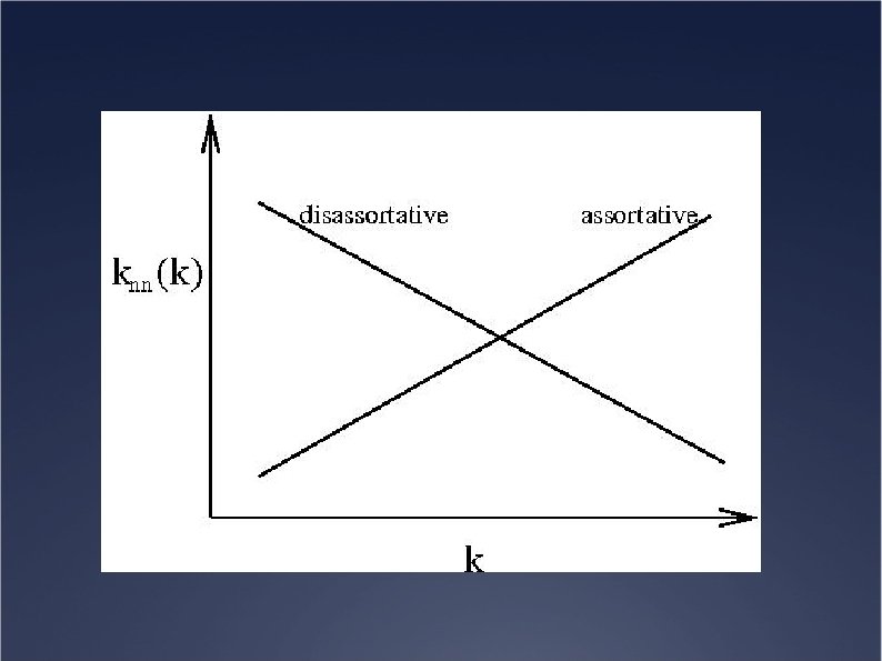
Typical correlations Ü Assortative behaviour: growing knn(k) Example: social networks Large sites are connected with large sites Ü Disassortative behaviour: decreasing knn(k) Example: internet Large sites connected with small sites, hierarchical structure

Correlations: Clustering spectrum • P(k’, k’’|k): cumbersome, difficult to estimate from data • Average clustering coefficient C=average over vertices with very different characteristics Clustering spectrum: putting together vertices which have the same degree class of degree k (link with hierarchical structures)

Motifs: subgraphs occurring more often than on random versions of the graph Significance of motifs: Z-score!

Weighted networks Real world networks: edges Ü carry traffic (transport networks, Internet…) Ü have different intensities (social networks…) General description: weights i wij j aij: 0 or 1 wij: continuous variable

Weights: examples ● Scientific collaborations: number of common papers ● Internet, emails: traffic, number of exchanged emails ● Airports: number of passengers ● Metabolic networks: fluxes ● … usually wii=0 symmetric: wij=wji

Weighted networks Weights: on the edges Strength of a vertex: si = j ε V(i) wij =>Naturally generalizes the degree to weighted networks =>Quantifies for example the total traffic at a vertex

Weighted clustering coefficient I i wij=1 i wij=5 A. Barrat, M. Barthélemy, R. Pastor-Satorras, A. Vespignani, PNAS 101, 3747 (2004) si=16 ciw=0. 625 > ci ki=4 ci=0. 5 si=8 ciw=0. 25 < ci

Weighted clustering coefficient II Definition based on subgraph intensity J. Saramäki, M. Kivela, J. -P. Onnela, K. Kaski, J. Kertész, Phys. Rev. E 75, 027105 (2007)

Weighted clustering coefficient wik Average clustering coefficient C= i C(i)/n Cw= i Cw(i)/n Random(ized) weights: C = Cw C < Cw : more weights on cliques C > Cw : less weights on cliques Clustering spectra

Weighted assortativity ki=5; knn, i=1. 8

Weighted assortativity 1 1 1 5 i 1 ki=5; knn, i=1. 8

Weighted assortativity 5 5 5 1 i 5 ki=5; si=21; knn, i=1. 8 ; knn, iw=1. 2: knn, i > knn, iw

Weighted assortativity 1 1 5 1 i 1 ki=5; si=9; knn, i=1. 8 ; knn, iw=3. 2: knn, i < knn, iw

Participation ratio 1/ki if all weights equal close to 1 if few weights dominate

Plan of the course I. Networks: definitions, characteristics, basic concepts in graph theory II. Real world networks: basic properties III. Models IV. Community structure II VI. Dynamic processes in networks