Lecture 9 TimeResponses of ClosedLoop SampleData Systems System

Lecture 9: Time-Responses of Closed-Loop Sample-Data Systems • System time-response • Characteristic equations and closed-loop poles • Dominant close-loop poles • Reading: Chapter 6 (except 6. 4)

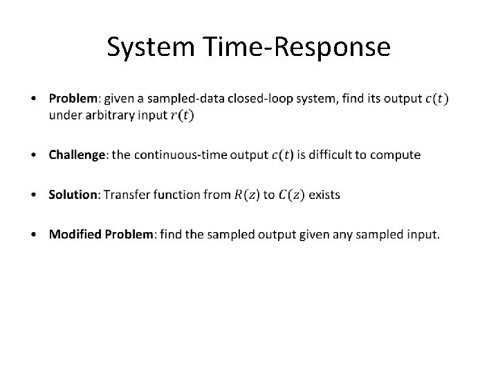
System Time-Response •

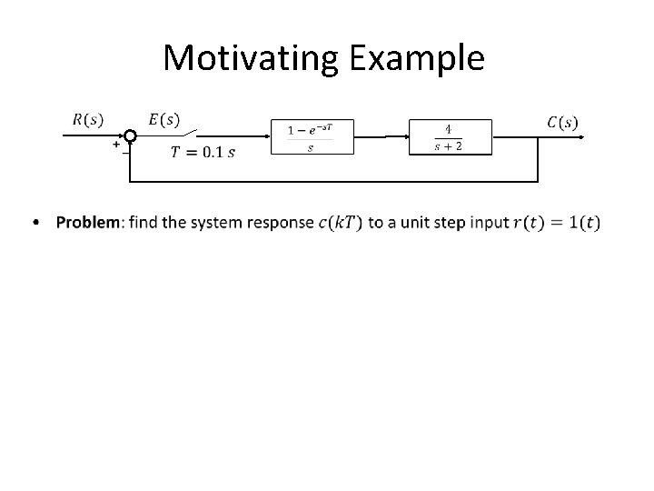
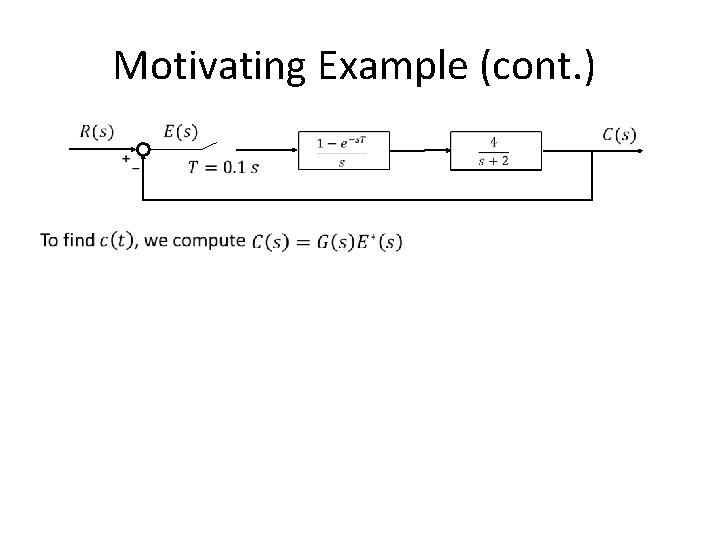
Motivating Example •

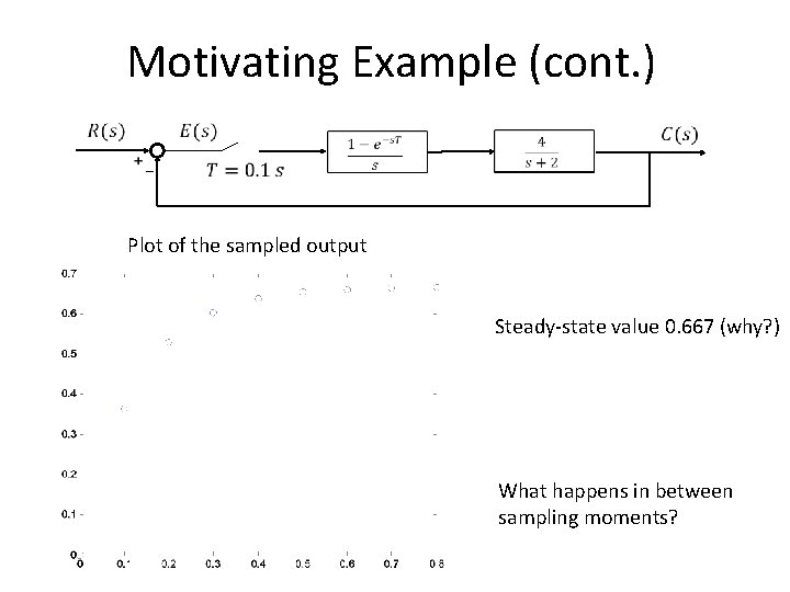
Motivating Example (cont. ) Plot of the sampled output Steady-state value 0. 667 (why? ) What happens in between sampling moments?

Motivating Example (cont. )

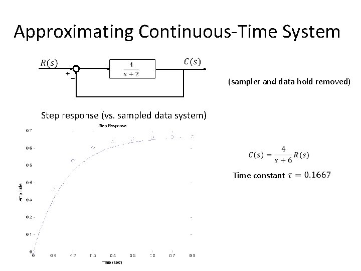
Approximating Continuous-Time System (sampler and data hold removed) Step response (vs. sampled data system) Time constant

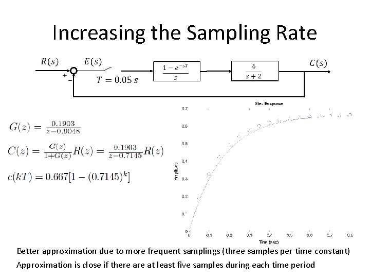
Increasing the Sampling Rate Better approximation due to more frequent samplings (three samples per time constant) Approximation is close if there at least five samples during each time period

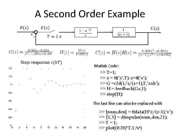
A Second Order Example Matlab Code: >> T=1; >> z = tf(‘z’, T); s=tf(‘s’); >> G =c 2 d(1/s/(s+1), T, ’zoh’); >> H = feedback(Gz, 1); >> step(H); The last line can also be replaced with >> [num, den] = tfdata(H*z/(z-1), ’v’); >> [Y, X] = dimpulse(num, den, 21); >> T = 1; >> plot((0: 20)*T, Y, 'o')

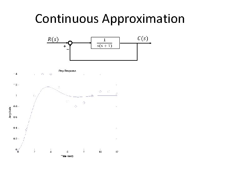
Continuous Approximation

Discussions • The final value of the sampled-data system agree with that of the continuous-time approximating system • Maximum overshoot is larger for the sampled-data system • Samplings seem to make the closed-loop system less “stable” • Discrepancy can be reduced by increasing the sampling rate

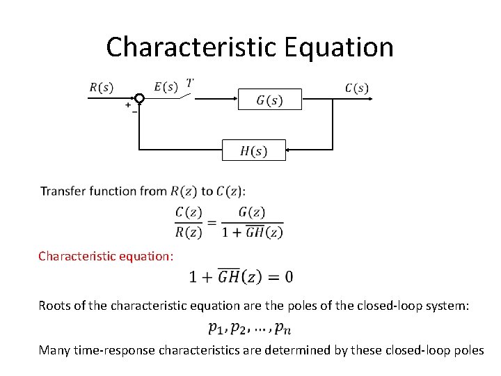
Characteristic Equation Characteristic equation: Roots of the characteristic equation are the poles of the closed-loop system: Many time-response characteristics are determined by these closed-loop poles

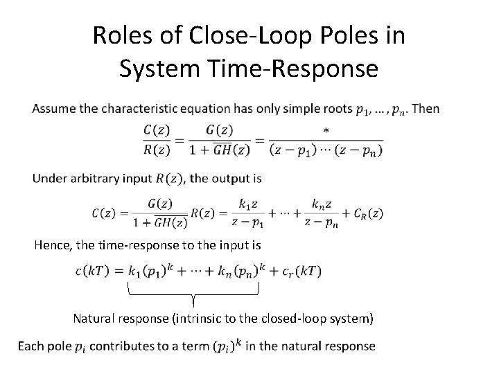
Roles of Close-Loop Poles in System Time-Response Hence, the time-response to the input is Natural response (intrinsic to the closed-loop system)

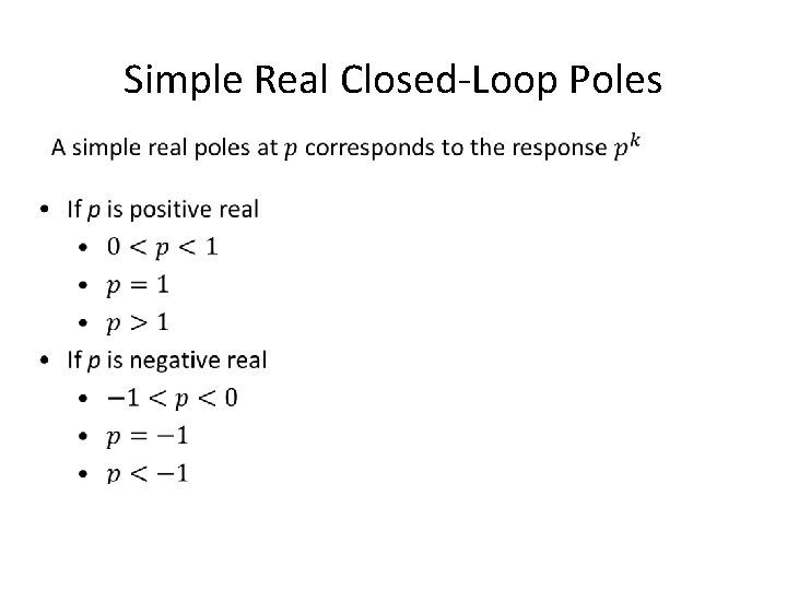
Simple Real Closed-Loop Poles

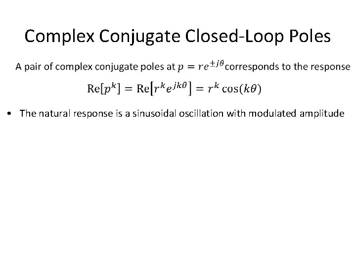
Complex Conjugate Closed-Loop Poles • The natural response is a sinusoidal oscillation with modulated amplitude

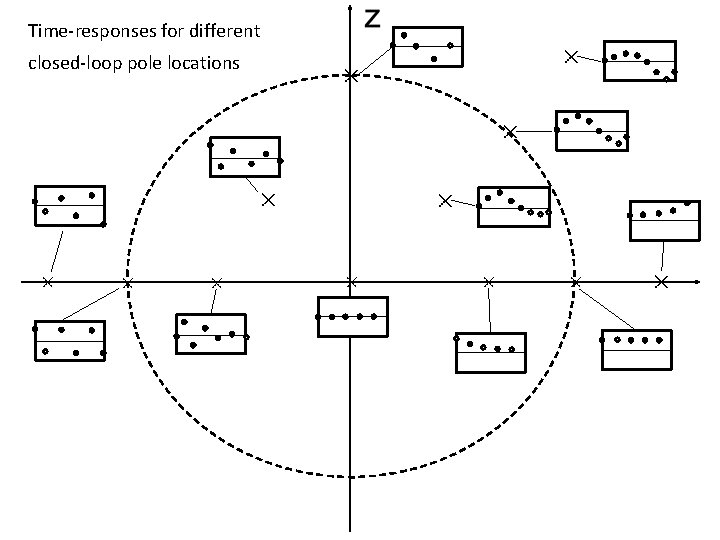
Time-responses for different closed-loop pole locations

Stable Systems • The closed-loop system is called stable if all its closed-loop poles are strictly inside the unit circle on the z-plane: • For a stable system, the natural response will eventually vanish; hence it is called the transient response in this case. • We will study stability more systematically later.

Dominant Closed-Loop Poles •

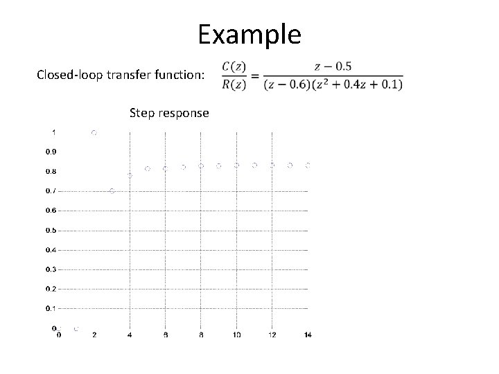
Example Closed-loop transfer function: Step response