Lecture 9 Smoothing and filtering data Time series


)*exp(-(x 0 -50)^2/(2*sig^2)) plot(x 0, y 0, type=\"l\", col=\"green\",")


. Locally-weighted least-squares (“lowess”, “loess”): fit a polynomial (usually a straight")


? Residuals? Events ?")

 penalized splines (akima’s aspline)")
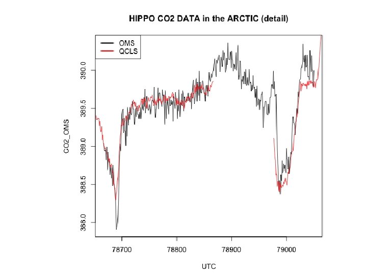
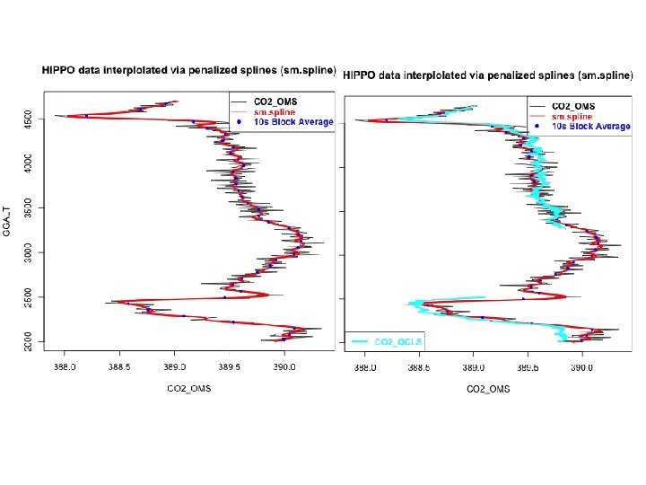
![XX=HIPPO. 1. 1[lsel&l. uct, "UTC"] YY=HIPPO. 1. 1[lsel&l. uct, "CO 2_OMS"] ZZ=HIPPO. 1. 1[lsel&l.](https://slidetodoc.com/presentation_image_h/83df777fc928ef6bc7055207399057a9/image-29.jpg "XX=HIPPO. 1. 1[lsel&l. uct, \"UTC\"] YY=HIPPO. 1. 1[lsel&l. uct, \"CO 2_OMS\"] ZZ=HIPPO. 1. 1[lsel&l.")


- Slides: 31
Lecture 9: Smoothing and filtering data
Time series: smoothing, filtering, rejecting outliers, interpolation moving average, splines, penalized splines, wavelets autocorrelation in time series variance increase, pattern generation; ar(), arima() … Image data
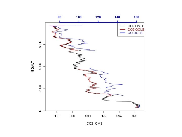
-- OMS -- QCLS
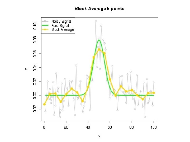
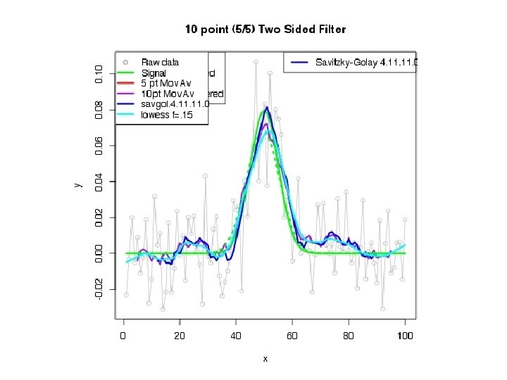
sig=5 x 0=1: 100; y 0=1/(sig*sqrt(2*pi))*exp(-(x 0 -50)^2/(2*sig^2)) plot(x 0, y 0, type="l", col="green", lwd=3, ylim=c(-. 02, . 1)) #add noise to y 0 x=x 0; y=y 0+rnorm(100)/50 points(x, y, pch=16, type="o”)
--- 5 pt moving average
--- 30 pt moving average
Some signal filtering concepts:
“What is” “feed-forward”?
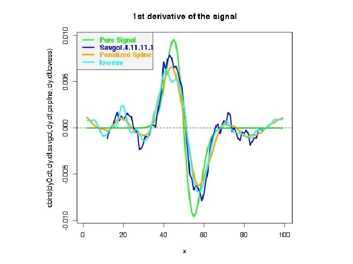
More advanced filters. Splines: Splines use a collection of basis functions (usually polynomials of order 3 or 4) to represent a functional form for the time series to be filtered. They are fitted piecewise, so that they are locally determined. We choose K points in the interior of the domain (“knots”) and subdivide into K+1 intervals. spline of order m: piecewise m – 1 degree polynomial, continuous thru m – 2 derivatives. Continuous derivatives gives a smooth function. More complex shapes emerge as we increase the degree of the spline and/or add knots. • Few knots/low degree: Functions may be too restrictive (biased) or smooth • Many knots/high degree: Risk of overfitting, false maxima, etc Penalized Splines add a penalty for curvature, specifying the strength λ. (=0, regular spline/interpolation; = ∞, straight line, linear regression fit)
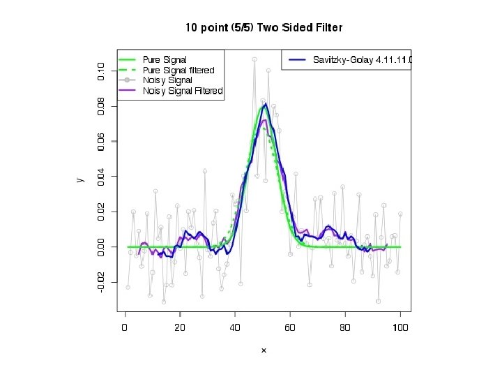
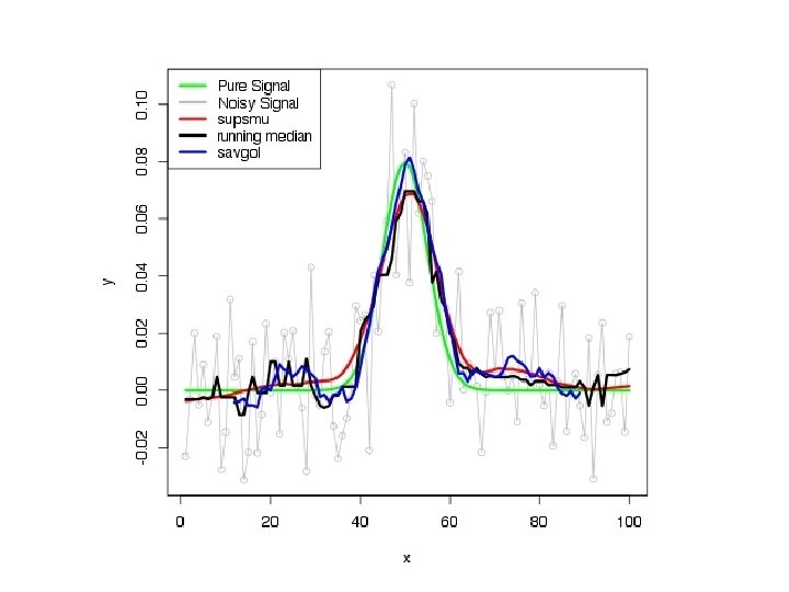
More advanced filters (continued). Locally-weighted least-squares (“lowess”, “loess”): fit a polynomial (usually a straight line) to points in a sliding window, accepting as the smoothed value the central point on the line, with a taper to capture the ends. Points are usually weighted inversely as a function of distance, very often tri-cubic: (1 - |x|3)3 <in range -1, 1 of the window> Savitsky-Golay filter: Fits a polynomial of order n in a moving window, requiring that the fitted curve at each point have the same moments as the original data to order n-1. Partakes of lowess and penalized spline features. (Designed for integrating chromatographic peaks. ) Nomencature: 4. 11. 0 ( n. nl. nr. o). Allows direct computation of the derivatives. Parameters are tabulated on the web or computed.
sig noisy_sig 10 -point MA savgol. 4. 11. 0 lowess pspline supsmu 0. 010 0. 012 NA NA 0. 0117 0. 0124 0. 010 0. 012 0. 0132 0. 0155 0. 0117 0. 0124
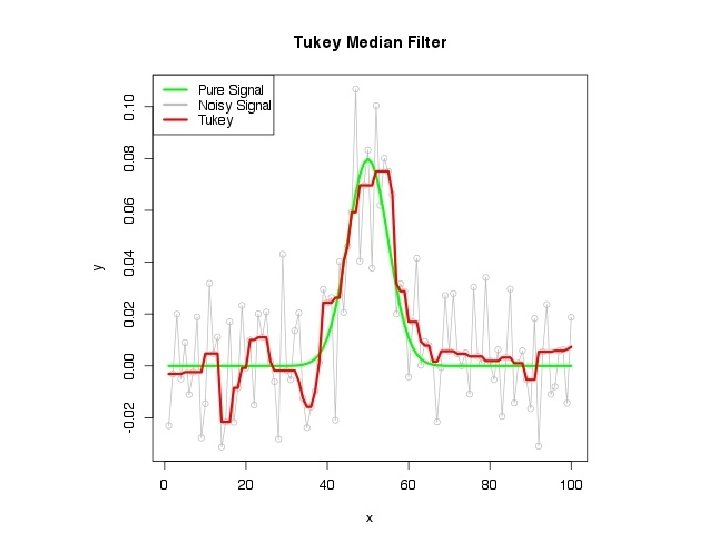
#Summary: #X Moving Average: crude, phase shift, peaks severely flattened, ends discarded <Don't use> ## Centered Moving Average: crude, peaks severely flattened, no phase shift*, feed forward >, ends discarded ## Block Averages: not too crude, not phase shifted*, no feed forward*, conserved properties*, information discarded (Maybe OK) ##Savitzky-Golay: not crude, not phase shifted*, small feed forward (localized), conserved properties, ends discarded; derivative ##locally weighted least squares (lowess/loess): not crude or phase shifted, nice taper at ends, no derivative ##supsmu: analytical properties murky, but a nice smoother for many signals; no derivative ##penalized splines: effective, differentiable; adjusting the parameters may be tricky #Xregular splines: either false maxima, or oversmoothed--<Don't use>
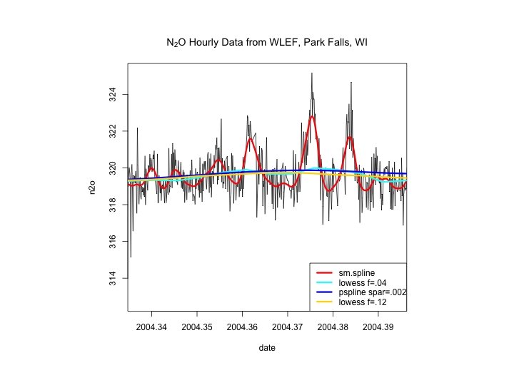
EPS 236 Workshop: 2014 Assessing different sources of variance: Extracting Trends, Cycles, etc by Data Filtering and Conditional Averaging. CO 2 Measurement has low signal-tonoise ratio. Measurement has high signal-to-noise ratio, but the system (e. g. the atmosphere) has a lot of variability.
“Ancillary measurements”, conditional sampling and suitable filtering or averaging reveals the key features of the data when system variability is the key factor. Zum=tapply(wlef[, "value"], list(wlef[, "yr"], wlef[, "mo"], wlef[, "hr"], wlef[, "ht(magl)"]), median, na. rm=T)
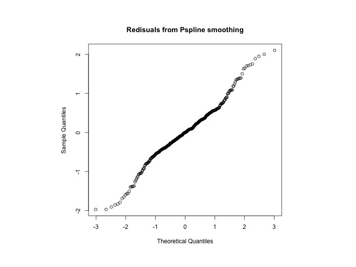
Noisy data: which filter is the “best” (for what purpose? )? Residuals? Events ?
If spar is given: Leave-one-out cross-validation In the default mode, the sm. spline model is selected using “leave-one-out cross-validation”. See article by Rob Hyndman (http: //robjhyndman. com/hyndsight/crossvalidation/) for a description. Kalman filter
Interpolation: linear (approx; predict. loess) penalized splines (akima’s aspline)
XX=HIPPO. 1. 1[lsel&l. uct, "UTC"] YY=HIPPO. 1. 1[lsel&l. uct, "CO 2_OMS"] ZZ=HIPPO. 1. 1[lsel&l. uct, "CO 2_QCLS"] YY[1379: 1387] = NA require(pspline) lna 1=!is. na(YY) YY. i=approx(x=XX[lna 1], y=YY[lna 1], xout=XX) YY. spl=sm. spline(XX[lna 1], YY[lna 1]) require(akima) YY. aspline= aspline(XX[lna 1], YY[lna 1], xout=XX) #YY. lowess=lowess(XX[lna 1], YY[lna 1], f=. 1) ddd=data. frame(x=XX[lna 1], y=YY[lna 1]) YY. loess=loess(y ~ x, data=ddd, span=. 055) YY. loess. pred=predict(YY. loess, newdata=data. frame(x=XX, y=YY))
“Leave-one-out” CV Source: http: //robjhyndman. com/hyndsight/crossvalidation/ Minimize CV for “best” model