Lecture 9 Convolutional Neural Networks 2 CS 109

Lecture 9: Convolutional Neural Networks 2 CS 109 B Data Science 2 Pavlos Protopapas and Mark Glickman 1

Outline 1. Review from last lecture 2. Back. Prop of Max. Pooling layer 3. A bit of history 4. Layers Receptive Field 5. Saliency maps 6. Transfer Learning 7. CNN for text analysis (example) CS 109 B, PROTOPAPAS, GLICKMAN 2

Outline 1. Review from last lecture 2. Back. Prop of Max. Pooling layer 3. A bit of history 4. Layers Receptive Field 5. Saliency maps 6. Transfer Learning 7. CNN for text analysis (example) CS 109 B, PROTOPAPAS, GLICKMAN 3

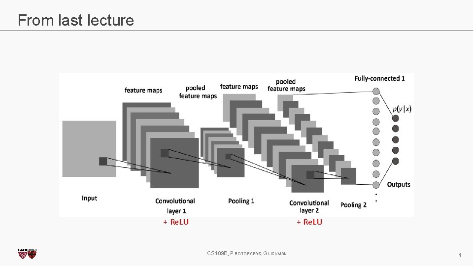
From last lecture + Re. LU CS 109 B, PROTOPAPAS, GLICKMAN 4

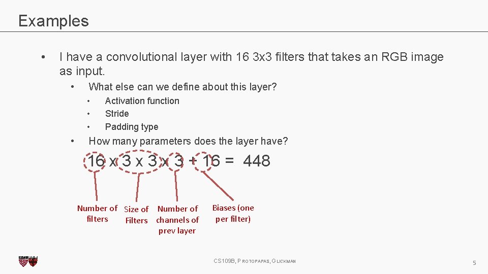
Examples • I have a convolutional layer with 16 3 x 3 filters that takes an RGB image as input. • What else can we define about this layer? • • Activation function Stride Padding type How many parameters does the layer have? 16 x 3 x 3 + 16 = 448 Number of Size of Number of filters Filters channels of prev layer Biases (one per filter) CS 109 B, PROTOPAPAS, GLICKMAN 5

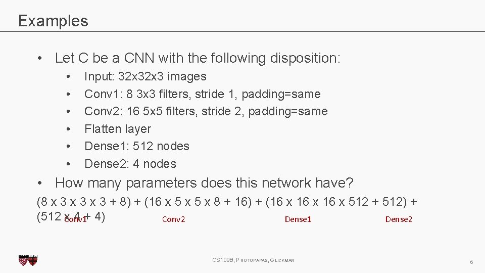
Examples • Let C be a CNN with the following disposition: • • • Input: 32 x 3 images Conv 1: 8 3 x 3 filters, stride 1, padding=same Conv 2: 16 5 x 5 filters, stride 2, padding=same Flatten layer Dense 1: 512 nodes Dense 2: 4 nodes • How many parameters does this network have? (8 x 3 x 3 + 8) + (16 x 5 x 8 + 16) + (16 x 512 + 512) + (512 x 4 + 4) Conv 1 Conv 2 Dense 1 Dense 2 CS 109 B, PROTOPAPAS, GLICKMAN 6

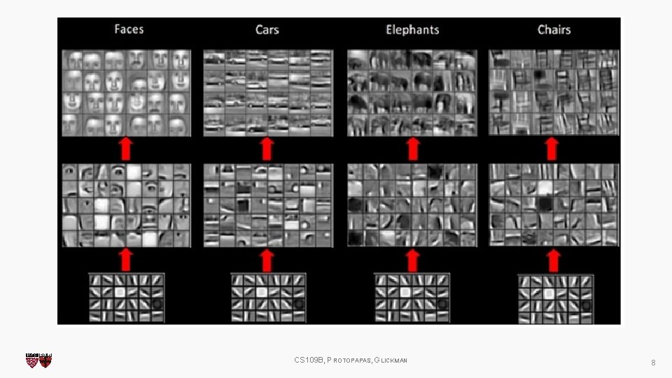
What do CNN layers learn? • Each CNN layer learns filters of increasing complexity. • The first layers learn basic feature detection filters: edges, corners, etc. • The middle layers learn filters that detect parts of objects. For faces, they might learn to respond to eyes, noses, etc. • The last layers have higher representations: they learn to recognize full objects, in different shapes and positions. CS 109 B, PROTOPAPAS, GLICKMAN 7

CS 109 B, PROTOPAPAS, GLICKMAN 8

3 D visualization of networks in action http: //scs. ryerson. ca/~aharley/vis/conv/ https: //www. youtube. com/watch? v=3 JQ 3 h. Yko 51 Y CS 109 B, PROTOPAPAS, GLICKMAN 9

Outline 1. Review from last lecture 2. Back. Prop of Max. Pooling layer 3. A bit of history 4. Layers Receptive Field 5. Saliency maps 6. Transfer Learning 7. CNN for text analysis (example) CS 109 B, PROTOPAPAS, GLICKMAN 10

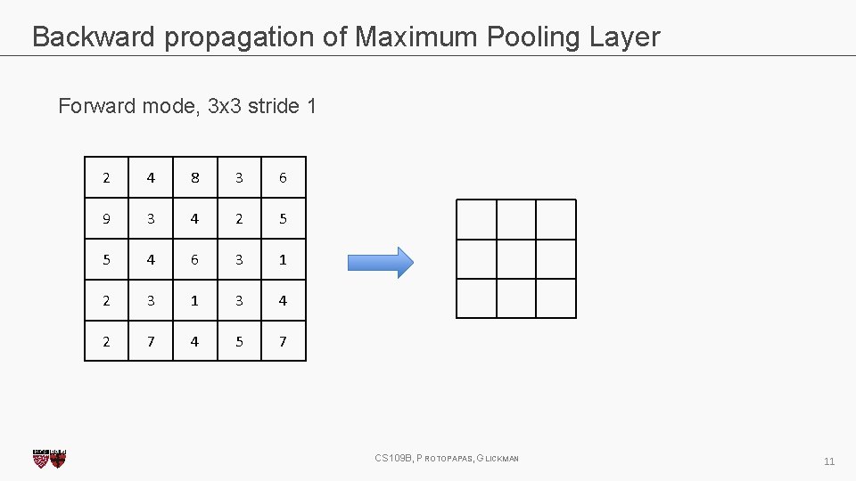
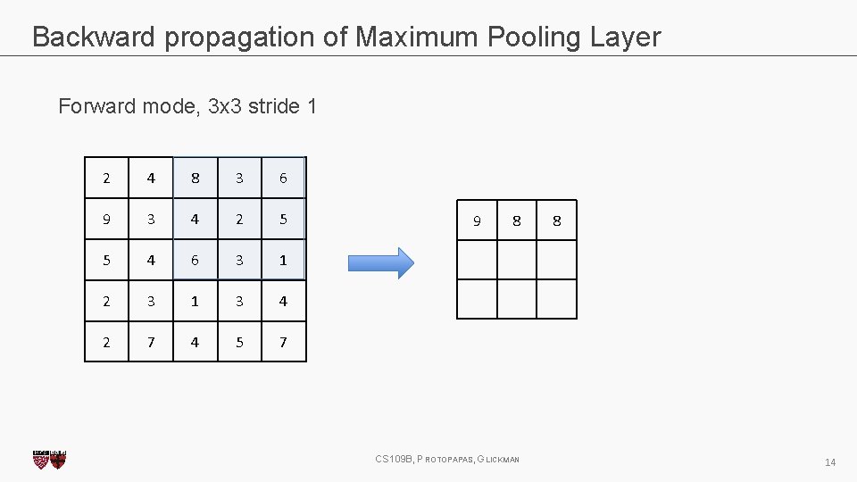
Backward propagation of Maximum Pooling Layer Forward mode, 3 x 3 stride 1 2 4 8 3 6 9 3 4 2 5 5 4 6 3 1 2 3 1 3 4 2 7 4 5 7 CS 109 B, PROTOPAPAS, GLICKMAN 11

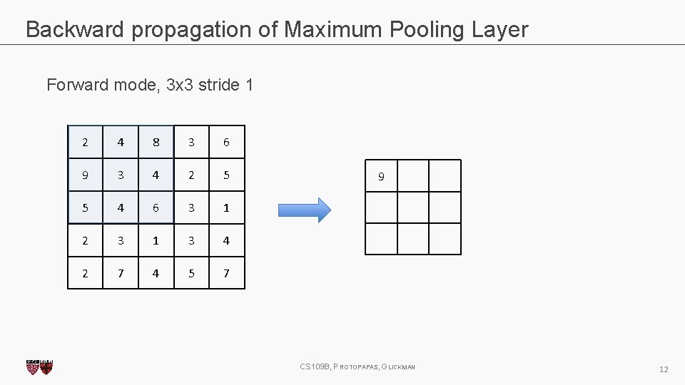
Backward propagation of Maximum Pooling Layer Forward mode, 3 x 3 stride 1 2 4 8 3 6 9 3 4 2 5 5 4 6 3 1 2 3 1 3 4 2 7 4 5 7 9 CS 109 B, PROTOPAPAS, GLICKMAN 12

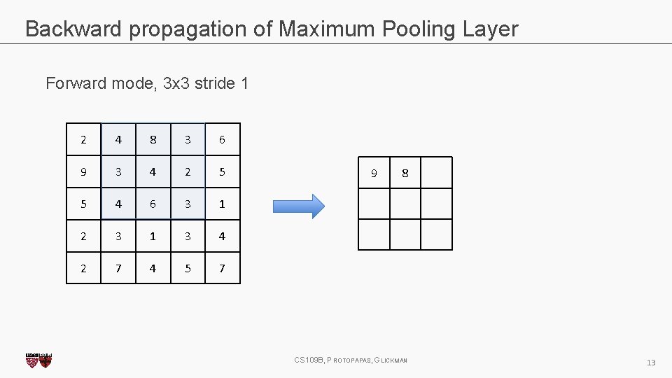
Backward propagation of Maximum Pooling Layer Forward mode, 3 x 3 stride 1 2 4 8 3 6 9 3 4 2 5 5 4 6 3 1 2 3 1 3 4 2 7 4 5 7 9 8 CS 109 B, PROTOPAPAS, GLICKMAN 13

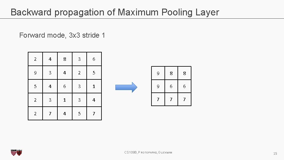
Backward propagation of Maximum Pooling Layer Forward mode, 3 x 3 stride 1 2 4 8 3 6 9 3 4 2 5 5 4 6 3 1 2 3 1 3 4 2 7 4 5 7 9 8 CS 109 B, PROTOPAPAS, GLICKMAN 8 14

Backward propagation of Maximum Pooling Layer Forward mode, 3 x 3 stride 1 2 4 8 3 6 9 3 4 2 5 9 8 8 5 4 6 3 1 9 6 6 2 3 1 3 4 7 7 7 2 7 4 5 7 CS 109 B, PROTOPAPAS, GLICKMAN 15

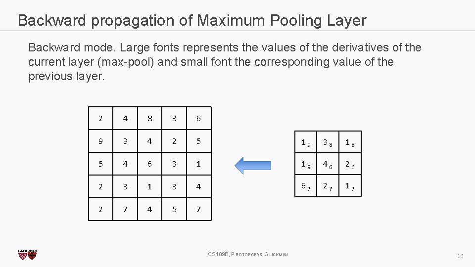
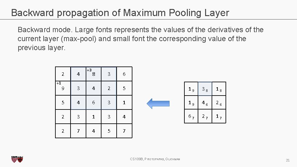
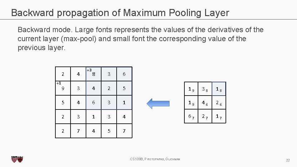
Backward propagation of Maximum Pooling Layer Backward mode. Large fonts represents the values of the derivatives of the current layer (max-pool) and small font the corresponding value of the previous layer. 2 4 8 3 6 9 3 4 2 5 1 9 3 8 1 8 5 4 6 3 1 1 9 4 6 2 3 1 3 4 6 7 2 7 1 7 2 7 4 5 7 CS 109 B, PROTOPAPAS, GLICKMAN 16

Backward propagation of Maximum Pooling Layer Backward mode. Large fonts represents the values of the derivatives of the current layer (max-pool) and small font the corresponding value of the previous layer. 2 4 8 3 6 9 3 4 2 5 1 9 3 8 1 8 5 4 6 3 1 1 9 4 6 2 3 1 3 4 6 7 2 7 1 7 2 7 4 5 7 CS 109 B, PROTOPAPAS, GLICKMAN 17

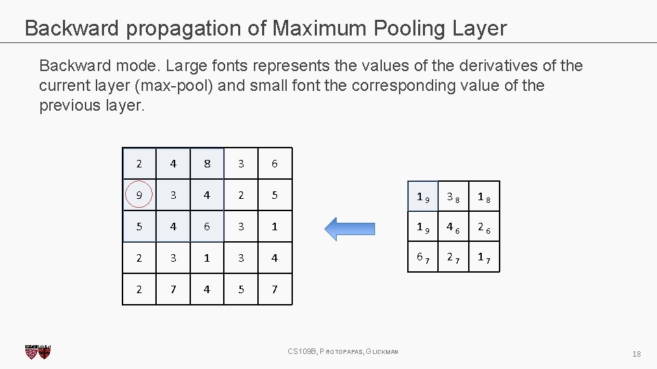
Backward propagation of Maximum Pooling Layer Backward mode. Large fonts represents the values of the derivatives of the current layer (max-pool) and small font the corresponding value of the previous layer. 2 4 8 3 6 9 3 4 2 5 1 9 3 8 1 8 5 4 6 3 1 1 9 4 6 2 3 1 3 4 6 7 2 7 1 7 2 7 4 5 7 CS 109 B, PROTOPAPAS, GLICKMAN 18

Backward propagation of Maximum Pooling Layer Backward mode. Large fonts represents the values of the derivatives of the current layer (max-pool) and small font the corresponding value of the previous layer. +1 2 4 8 3 6 9 3 4 2 5 1 9 3 8 1 8 5 4 6 3 1 1 9 4 6 2 3 1 3 4 6 7 2 7 1 7 2 7 4 5 7 CS 109 B, PROTOPAPAS, GLICKMAN 19

Backward propagation of Maximum Pooling Layer Backward mode. Large fonts represents the values of the derivatives of the current layer (max-pool) and small font the corresponding value of the previous layer. +1 2 4 8 3 6 9 3 4 2 5 1 9 3 8 1 8 5 4 6 3 1 1 9 4 6 2 3 1 3 4 6 7 2 7 1 7 2 7 4 5 7 CS 109 B, PROTOPAPAS, GLICKMAN 20

Backward propagation of Maximum Pooling Layer Backward mode. Large fonts represents the values of the derivatives of the current layer (max-pool) and small font the corresponding value of the previous layer. +1 2 4 9 +3 8 3 6 3 4 2 5 1 9 3 8 1 8 5 4 6 3 1 1 9 4 6 2 3 1 3 4 6 7 2 7 1 7 2 7 4 5 7 CS 109 B, PROTOPAPAS, GLICKMAN 21

Backward propagation of Maximum Pooling Layer Backward mode. Large fonts represents the values of the derivatives of the current layer (max-pool) and small font the corresponding value of the previous layer. +1 2 4 9 +3 8 3 6 3 4 2 5 1 9 3 8 1 8 5 4 6 3 1 1 9 4 6 2 3 1 3 4 6 7 2 7 1 7 2 7 4 5 7 CS 109 B, PROTOPAPAS, GLICKMAN 22

Backward propagation of Maximum Pooling Layer Backward mode. Large fonts represents the values of the derivatives of the current layer (max-pool) and small font the corresponding value of the previous layer. +1 2 4 9 +3 8 3 6 3 4 2 5 1 9 3 8 1 8 5 4 6 3 1 1 9 4 6 2 3 1 3 4 6 7 2 7 1 7 2 7 4 5 7 CS 109 B, PROTOPAPAS, GLICKMAN 23

Backward propagation of Maximum Pooling Layer Backward mode. Large fonts represents the values of the derivatives of the current layer (max-pool) and small font the corresponding value of the previous layer. +1 2 4 9 +4 8 3 6 3 4 2 5 1 9 3 8 1 8 5 4 6 3 1 1 9 4 6 2 3 1 3 4 6 7 2 7 1 7 2 7 4 5 7 CS 109 B, PROTOPAPAS, GLICKMAN 24

Outline 1. Review from last lecture 2. Back. Prop of Max. Pooling layer 3. A bit of history 4. Layers Receptive Field 5. Saliency maps 6. Transfer Learning 7. CNN for text analysis (example) CS 109 B, PROTOPAPAS, GLICKMAN 25

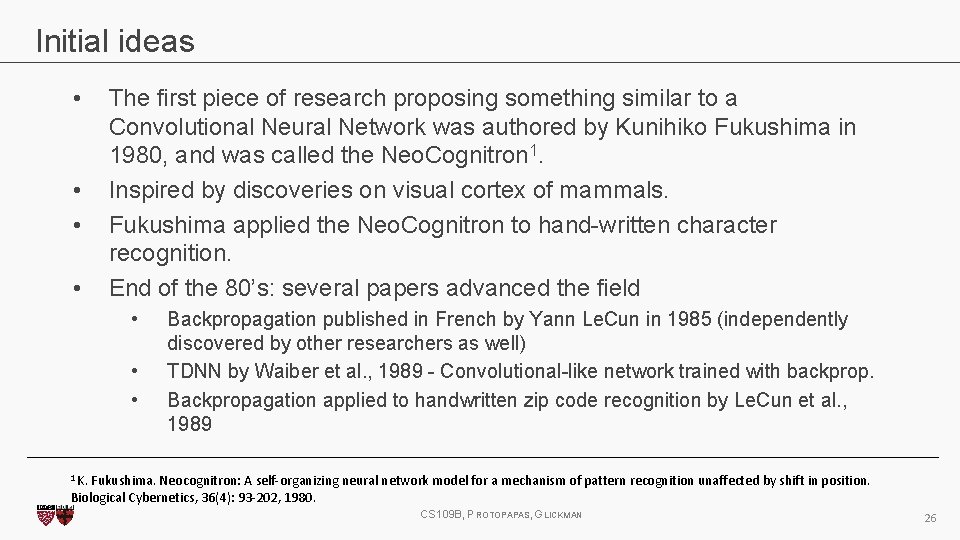
Initial ideas • • The first piece of research proposing something similar to a Convolutional Neural Network was authored by Kunihiko Fukushima in 1980, and was called the Neo. Cognitron 1. Inspired by discoveries on visual cortex of mammals. Fukushima applied the Neo. Cognitron to hand-written character recognition. End of the 80’s: several papers advanced the field • • • Backpropagation published in French by Yann Le. Cun in 1985 (independently discovered by other researchers as well) TDNN by Waiber et al. , 1989 - Convolutional-like network trained with backprop. Backpropagation applied to handwritten zip code recognition by Le. Cun et al. , 1989 1 K. Fukushima. Neocognitron: A self-organizing neural network model for a mechanism of pattern recognition unaffected by shift in position. Biological Cybernetics, 36(4): 93 -202, 1980. CS 109 B, PROTOPAPAS, GLICKMAN 26

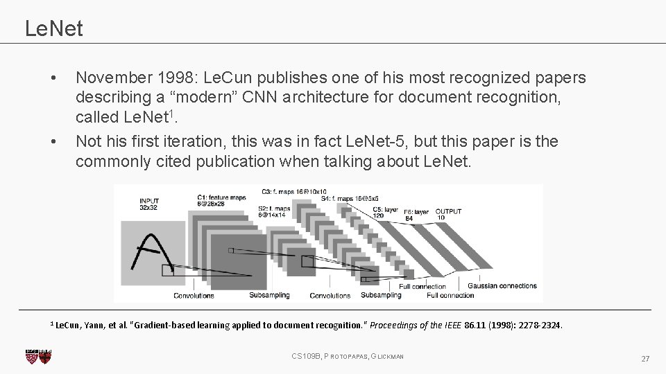
Le. Net • • November 1998: Le. Cun publishes one of his most recognized papers describing a “modern” CNN architecture for document recognition, called Le. Net 1. Not his first iteration, this was in fact Le. Net-5, but this paper is the commonly cited publication when talking about Le. Net. 1 Le. Cun, Yann, et al. "Gradient-based learning applied to document recognition. " Proceedings CS 109 B, PROTOPAPAS, GLICKMAN of the IEEE 86. 11 (1998): 2278 -2324. 27

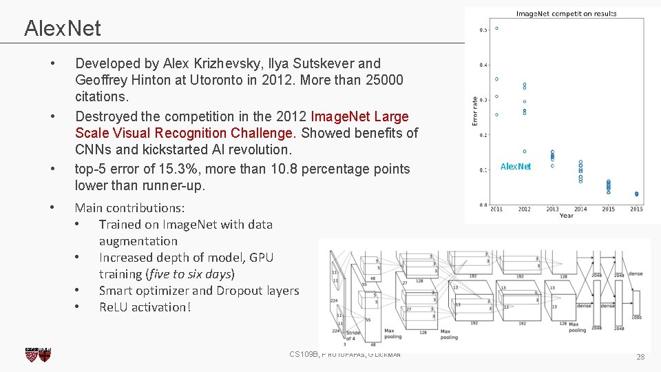
Alex. Net • • • Developed by Alex Krizhevsky, Ilya Sutskever and Geoffrey Hinton at Utoronto in 2012. More than 25000 citations. Destroyed the competition in the 2012 Image. Net Large Scale Visual Recognition Challenge. Showed benefits of CNNs and kickstarted AI revolution. top-5 error of 15. 3%, more than 10. 8 percentage points lower than runner-up. Alex. Net • Main contributions: • Trained on Image. Net with data augmentation • Increased depth of model, GPU training (five to six days) • Smart optimizer and Dropout layers • Re. LU activation! CS 109 B, PROTOPAPAS, GLICKMAN 28

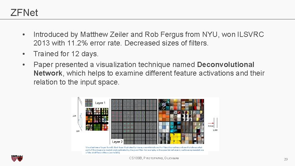
ZFNet • • • Introduced by Matthew Zeiler and Rob Fergus from NYU, won ILSVRC 2013 with 11. 2% error rate. Decreased sizes of filters. Trained for 12 days. Paper presented a visualization technique named Deconvolutional Network, which helps to examine different feature activations and their relation to the input space. CS 109 B, PROTOPAPAS, GLICKMAN 29

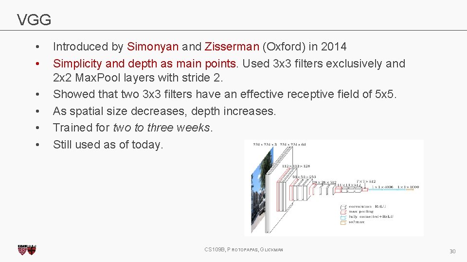
VGG • • • Introduced by Simonyan and Zisserman (Oxford) in 2014 Simplicity and depth as main points. Used 3 x 3 filters exclusively and 2 x 2 Max. Pool layers with stride 2. Showed that two 3 x 3 filters have an effective receptive field of 5 x 5. As spatial size decreases, depth increases. Trained for two to three weeks. Still used as of today. CS 109 B, PROTOPAPAS, GLICKMAN 30

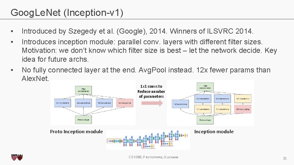
Goog. Le. Net (Inception-v 1) • • • Introduced by Szegedy et al. (Google), 2014. Winners of ILSVRC 2014. Introduces inception module: parallel conv. layers with different filter sizes. Motivation: we don’t know which filter size is best – let the network decide. Key idea for future archs. No fully connected layer at the end. Avg. Pool instead. 12 x fewer params than Alex. Net. 1 x 1 convs to Reduce number of parameters Proto Inception module CS 109 B, PROTOPAPAS, GLICKMAN 31

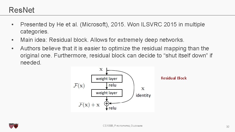
Res. Net • • • Presented by He et al. (Microsoft), 2015. Won ILSVRC 2015 in multiple categories. Main idea: Residual block. Allows for extremely deep networks. Authors believe that it is easier to optimize the residual mapping than the original one. Furthermore, residual block can decide to “shut itself down” if needed. Residual Block CS 109 B, PROTOPAPAS, GLICKMAN 32

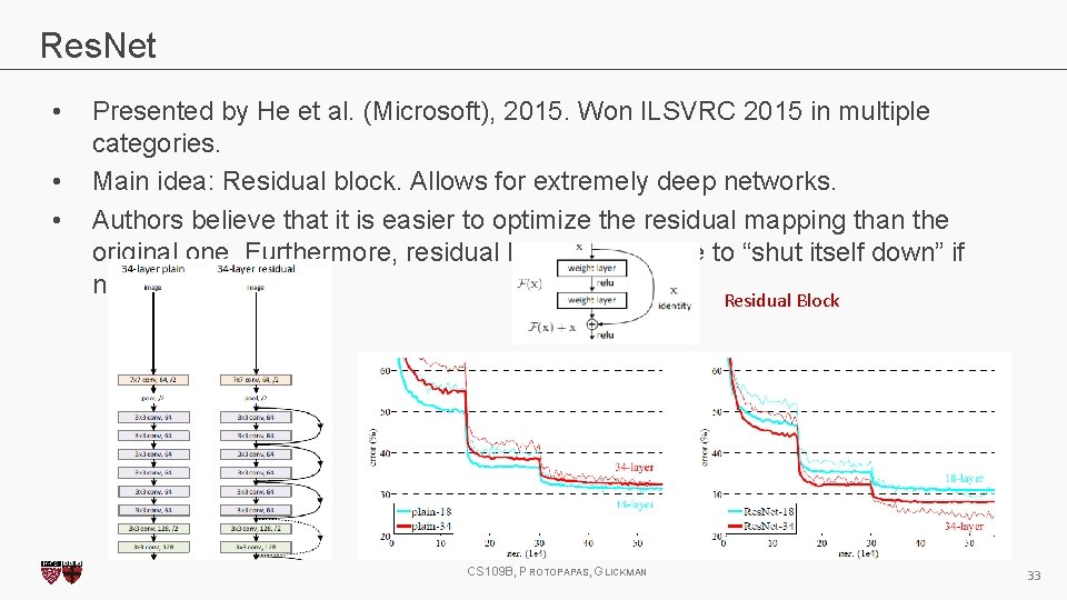
Res. Net • • • Presented by He et al. (Microsoft), 2015. Won ILSVRC 2015 in multiple categories. Main idea: Residual block. Allows for extremely deep networks. Authors believe that it is easier to optimize the residual mapping than the original one. Furthermore, residual block can decide to “shut itself down” if needed. Residual Block CS 109 B, PROTOPAPAS, GLICKMAN 33

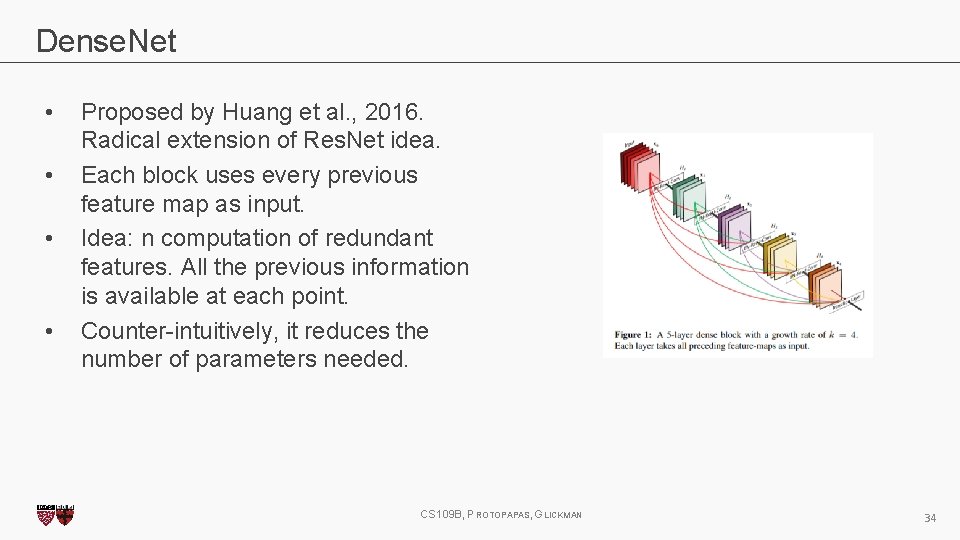
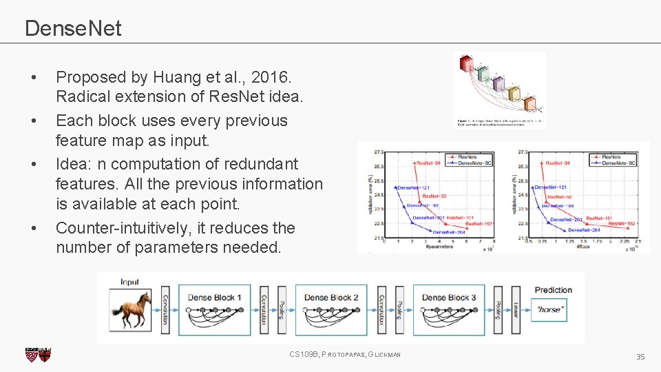
Dense. Net • • Proposed by Huang et al. , 2016. Radical extension of Res. Net idea. Each block uses every previous feature map as input. Idea: n computation of redundant features. All the previous information is available at each point. Counter-intuitively, it reduces the number of parameters needed. CS 109 B, PROTOPAPAS, GLICKMAN 34

Dense. Net • • Proposed by Huang et al. , 2016. Radical extension of Res. Net idea. Each block uses every previous feature map as input. Idea: n computation of redundant features. All the previous information is available at each point. Counter-intuitively, it reduces the number of parameters needed. CS 109 B, PROTOPAPAS, GLICKMAN 35

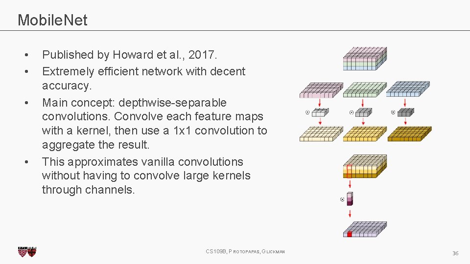
Mobile. Net • • Published by Howard et al. , 2017. Extremely efficient network with decent accuracy. Main concept: depthwise-separable convolutions. Convolve each feature maps with a kernel, then use a 1 x 1 convolution to aggregate the result. This approximates vanilla convolutions without having to convolve large kernels through channels. CS 109 B, PROTOPAPAS, GLICKMAN 36

More on the greatest latest at a-sec later today CS 109 B, PROTOPAPAS, GLICKMAN 37

Outline 1. Review from last lecture 2. Back. Prop of Max. Pooling layer 3. A bit of history 4. Layers Receptive Field 5. Saliency maps 6. Transfer Learning 7. CNN for text analysis (example) CS 109 B, PROTOPAPAS, GLICKMAN 38

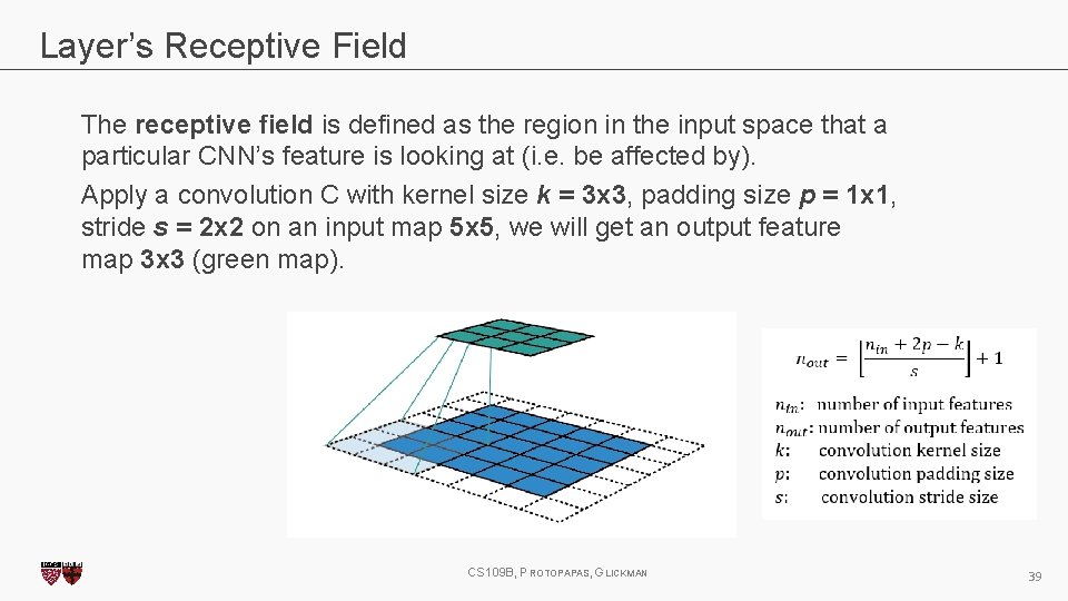
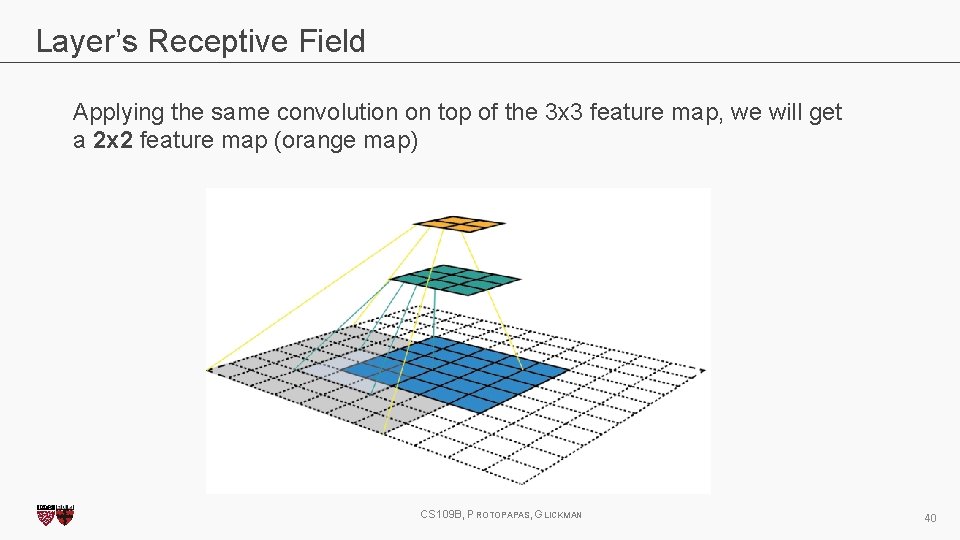
Layer’s Receptive Field The receptive field is defined as the region in the input space that a particular CNN’s feature is looking at (i. e. be affected by). Apply a convolution C with kernel size k = 3 x 3, padding size p = 1 x 1, stride s = 2 x 2 on an input map 5 x 5, we will get an output feature map 3 x 3 (green map). CS 109 B, PROTOPAPAS, GLICKMAN 39

Layer’s Receptive Field Applying the same convolution on top of the 3 x 3 feature map, we will get a 2 x 2 feature map (orange map) CS 109 B, PROTOPAPAS, GLICKMAN 40

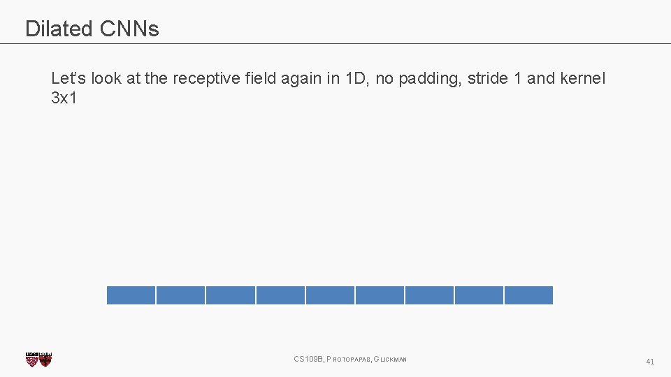
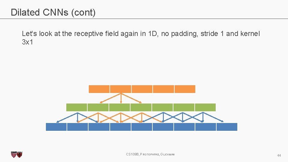
Dilated CNNs Let’s look at the receptive field again in 1 D, no padding, stride 1 and kernel 3 x 1 CS 109 B, PROTOPAPAS, GLICKMAN 41

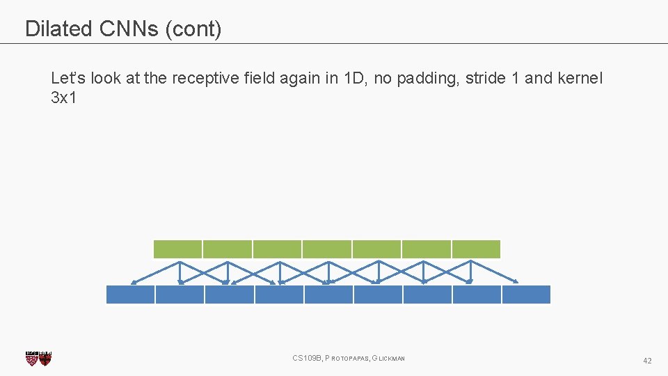
Dilated CNNs (cont) Let’s look at the receptive field again in 1 D, no padding, stride 1 and kernel 3 x 1 CS 109 B, PROTOPAPAS, GLICKMAN 42

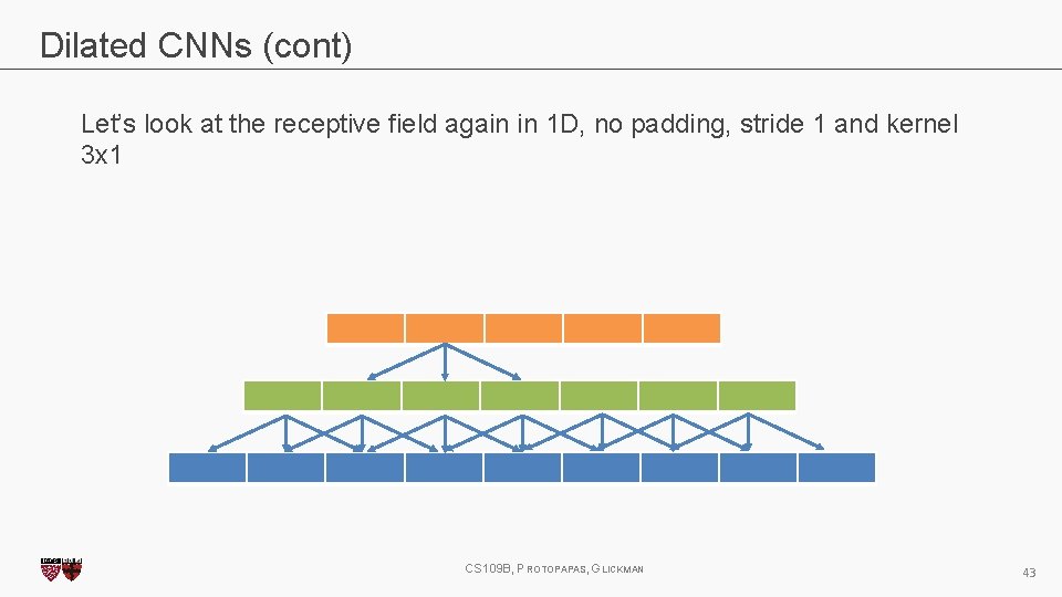
Dilated CNNs (cont) Let’s look at the receptive field again in 1 D, no padding, stride 1 and kernel 3 x 1 CS 109 B, PROTOPAPAS, GLICKMAN 43

Dilated CNNs (cont) Let’s look at the receptive field again in 1 D, no padding, stride 1 and kernel 3 x 1 CS 109 B, PROTOPAPAS, GLICKMAN 44

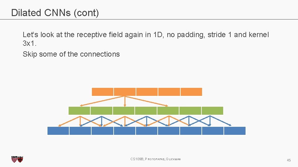
Dilated CNNs (cont) Let’s look at the receptive field again in 1 D, no padding, stride 1 and kernel 3 x 1. Skip some of the connections CS 109 B, PROTOPAPAS, GLICKMAN 45

Outline 1. Review from last lecture 2. Back. Prop of Max. Pooling layer 3. A bit of history 4. Layers Receptive Field 5. Saliency maps 6. Transfer Learning 7. CNN for text analysis (example) CS 109 B, PROTOPAPAS, GLICKMAN 46

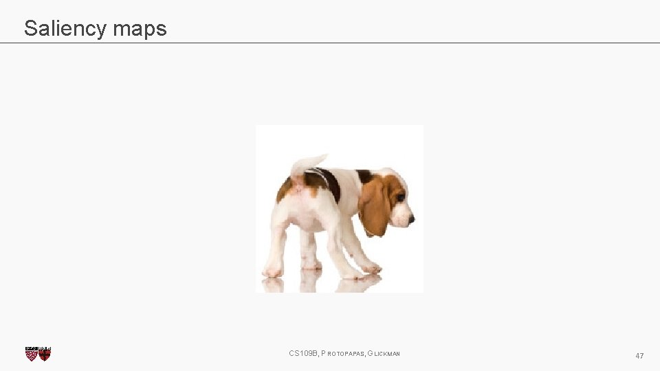
Saliency maps CS 109 B, PROTOPAPAS, GLICKMAN 47

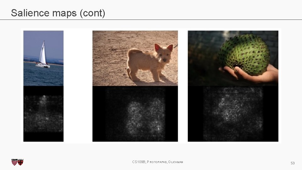
Saliency maps (cont) If you are given an image of a dog and asked to classify it. Most probably you will answer immediately – Dog! But your Deep Learning Network might not be as smart as you. It might classify it as a cat, a lion or Pavlos! What are the reasons for that? • bias in training data • no regularization • or your network has seen too many celebrities CS 109 B, PROTOPAPAS, GLICKMAN 48

Saliency maps (cont) We want to understand what made my network give a certain class as output? Saliency Maps, they are a way to measure the spatial support of a particular class in a given image. “Find me pixels responsible for the class C having score S(C) when the image I is passed through my network”. CS 109 B, PROTOPAPAS, GLICKMAN 49

Saliency maps (cont) We want to understand what made my network give a certain class as output? Saliency Maps, they are a way to measure the spatial support of a particular class in a given image. “Find me pixels responsible for the class C having score S(C) when the image I is passed through my network”. CS 109 B, PROTOPAPAS, GLICKMAN 50

Salience maps (cont) Question: How do we do that? We differentiate! For any function f(x, y, z), we can find the impact of variables x, y, z on fat any specific point (x 0, y 0, z 0) by finding its partial derivative w. r. t these variables at that point. Similarly, to find the responsible pixels, we take the score function S, for class C and take the partial derivatives w. r. t every pixel. CS 109 B, PROTOPAPAS, GLICKMAN 51

Salience maps (cont) Question: Easy Peasy? Sort of! Auto-grad can do this! 1. Forwar pass of the image through the network 2. Calculate the scores for every class 3. Enforce derivative of score S at last layer for all classes except class C to be 0. For C, set it to 1 4. Backpropagate this derivative till the start 5. Render them and you have your Saliency Map! Note: On step #2. Instead of doing softmax, we turn it to binary classification and use the probabilities. CS 109 B, PROTOPAPAS, GLICKMAN 52

Salience maps (cont) CS 109 B, PROTOPAPAS, GLICKMAN 53

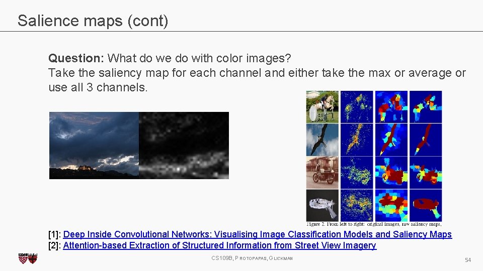
Salience maps (cont) Question: What do we do with color images? Take the saliency map for each channel and either take the max or average or use all 3 channels. [1]: Deep Inside Convolutional Networks: Visualising Image Classification Models and Saliency Maps [2]: Attention-based Extraction of Structured Information from Street View Imagery CS 109 B, PROTOPAPAS, GLICKMAN 54

Outline 1. Review from last lecture 2. Back. Prop of Max. Pooling layer 3. A bit of history 4. Layers Receptive Field 5. Saliency maps 6. Transfer Learning 7. CNN for text analysis (example) CS 109 B, PROTOPAPAS, GLICKMAN 55

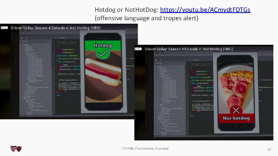
Transfer Learning How do you make an image classifier that can be trained in a few hours (minutes) on a CPU? Use pre-trained models, i. e. , models with known weights. Main Idea: earlier layers of a network learn low level features, which can be adapted to new domains by changing weights at later and fully-connected layers. Example: use Imagenet trained with any sophisticated huge network. Then retrain it on a few thousand hotdog images and you get. . . CS 109 B, PROTOPAPAS, GLICKMAN 56

Hotdog or Not. Hot. Dog: https: //youtu. be/ACmydt. FDTGs (offensive language and tropes alert) CS 109 B, PROTOPAPAS, GLICKMAN 57

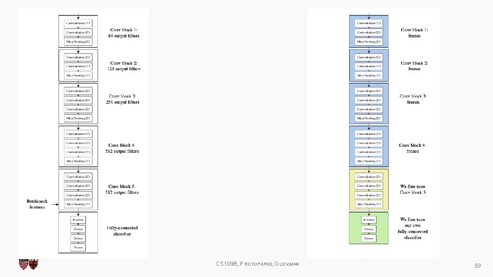
Transfer Learning (cont) 1. Get existing network weights 2. Un-freeze the “head” fully connected layers and train on your new images 3. Un-freeze the latest convolutional layers and train at a very low learning rate starting with the weights from the previously trained weights. This will change the latest layer convolutional weights without triggering large gradient updates which would have occurred had we not done 2. See https: //medium. com/@timanglade/how-hbos-silicon-valley-built-not-hotdog-with-mobiletensorflow-keras-react-native-ef 03260747 f 3 and https: //blog. keras. io/building-powerful-imageclassification-models-using-very-little-data. html for some details CS 109 B, PROTOPAPAS, GLICKMAN 58

CS 109 B, PROTOPAPAS, GLICKMAN 59

Outline 1. Review from last lecture 2. Back. Prop of Max. Pooling layer 3. A bit of history 4. Layers Receptive Field 5. Saliency maps 6. Transfer Learning 7. CNN for text analysis (example) CS 109 B, PROTOPAPAS, GLICKMAN 60

Convolutional Neural Networks for Text Classification When applied to text instead of images, we have an 1 dimensional array representing the text. Here the architecture of the Conv. Nets is changed to 1 D convolutional-and-pooling operations. One of the most typically tasks in NLP where Conv. Net are used is sentence classification, that is, classifying a sentence into a set of pre-determined categories by considering n-grams, i. e. it’s words or sequence of words, or also characters or sequence of characters. LETS SEE THIS THROUGH AN EXAMPLE CS 109 B, PROTOPAPAS, GLICKMAN 61

Beyond • Mobile. Net. V 2 (https: //arxiv. org/abs/1801. 04381) • Inception-Resnet, v 1 and v 2 (https: //arxiv. org/abs/1602. 07261) • Wide-Resnet (https: //arxiv. org/abs/1605. 07146) • Xception (https: //arxiv. org/abs/1610. 02357) • Res. Ne. Xt (https: //arxiv. org/pdf/1611. 05431) • Shuffle. Net, v 1 and v 2 (https: //arxiv. org/abs/1707. 01083) • Squeeze and Excitation Nets (https: //arxiv. org/abs/1709. 01507 ) CS 109 B, PROTOPAPAS, GLICKMAN 62