Lecture 9 Agenda Survival Analysis Part II Review

Lecture 9

Agenda • Survival Analysis (Part II) – Review basics – Cox Proportional Hazards Model – Accelerated Failure Time Models • Lognormal distribution • Weibull distribution

Review • A time to event outcome is defined as the following pair of variables: – Survival time T = min(event time, censoring time) – Event indicator d = 1 if event observed, 0 = if event is right censored • Right censoring is present in almost all applications. – Will focus primarily on time to event data with possible right censoring. – Left and interval censoring are uncommon in applications. Will not discuss these cases further.

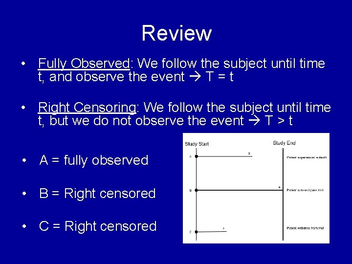
Review • Fully Observed: We follow the subject until time t, and observe the event T = t • Right Censoring: We follow the subject until time t, but we do not observe the event T > t • A = fully observed • B = Right censored • C = Right censored

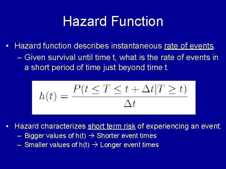
Review • Survival can be summarized as: – Median survival (value of t where S(t) =. 5) – Survival Function: S(t) = P(T > t) – Hazard Rate: h(t) = P(t ≤ T ≤ t+Δt | T ≥ t)/Δt • Nonparametric estimation of S(t) Kaplan-Meier – Calculate proportion at risk who died at time t – Multiply proportion remaining at time t-1 by proportion remaining at time t – Repeat for each unique event time – Subjects who are right censored are assumed not to be at risk beyond the time of censoring.

Hazard Function • Hazard function describes instantaneous rate of events. – Given survival until time t, what is the rate of events in a short period of time just beyond time t. • Hazard characterizes short term risk of experiencing an event. – Bigger values of h(t) Shorter event times – Smaller values of h(t) Longer event times

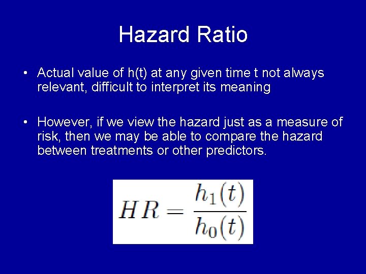
Hazard Ratio • Actual value of h(t) at any given time t not always relevant, difficult to interpret its meaning • However, if we view the hazard just as a measure of risk, then we may be able to compare the hazard between treatments or other predictors.

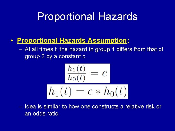
Proportional Hazards • Proportional Hazards Assumption: – At all times t, the hazard in group 1 differs from that of group 2 by a constant c. – Idea is similar to how one constructs a relative risk or an odds ratio.

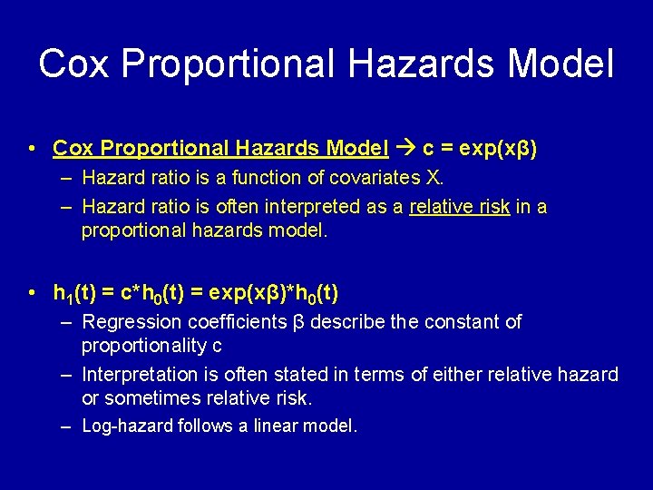
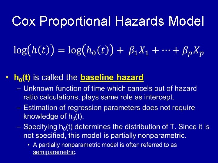
Cox Proportional Hazards Model • Cox Proportional Hazards Model c = exp(xβ) – Hazard ratio is a function of covariates X. – Hazard ratio is often interpreted as a relative risk in a proportional hazards model. • h 1(t) = c*h 0(t) = exp(xβ)*h 0(t) – Regression coefficients β describe the constant of proportionality c – Interpretation is often stated in terms of either relative hazard or sometimes relative risk. – Log-hazard follows a linear model.

Cox Proportional Hazards Model •

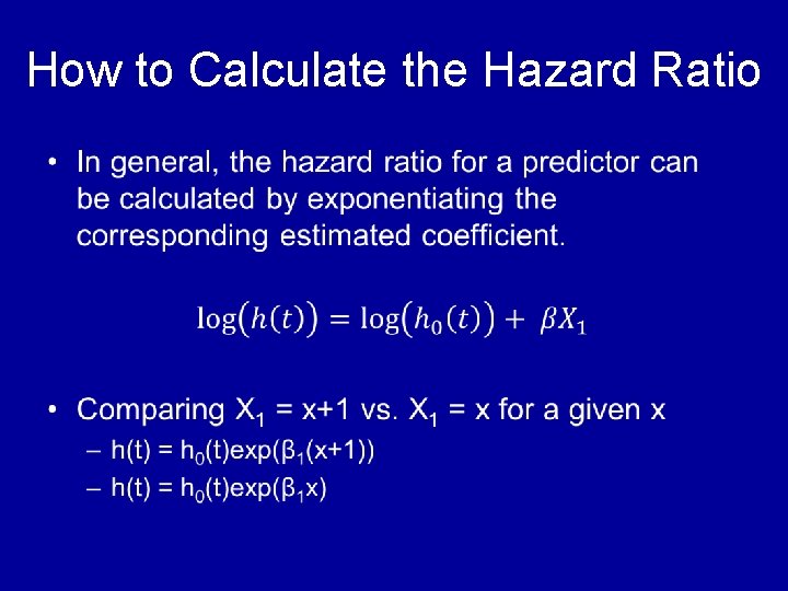
How to Calculate the Hazard Ratio •

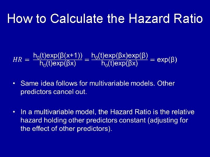
How to Calculate the Hazard Ratio •

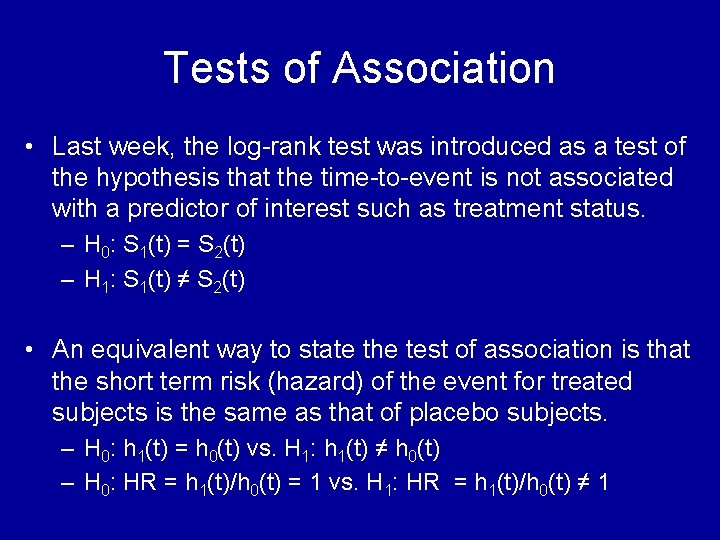
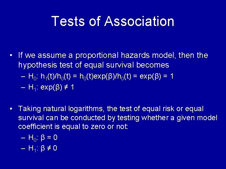
Tests of Association • Last week, the log-rank test was introduced as a test of the hypothesis that the time-to-event is not associated with a predictor of interest such as treatment status. – H 0: S 1(t) = S 2(t) – H 1: S 1(t) ≠ S 2(t) • An equivalent way to state the test of association is that the short term risk (hazard) of the event for treated subjects is the same as that of placebo subjects. – H 0: h 1(t) = h 0(t) vs. H 1: h 1(t) ≠ h 0(t) – H 0: HR = h 1(t)/h 0(t) = 1 vs. H 1: HR = h 1(t)/h 0(t) ≠ 1

Tests of Association • If we assume a proportional hazards model, then the hypothesis test of equal survival becomes – H 0: h 1(t)/h 0(t) = h 0(t)exp(β)/h 0(t) = exp(β) = 1 – H 1: exp(β) ≠ 1 • Taking natural logarithms, the test of equal risk or equal survival can be conducted by testing whether a given model coefficient is equal to zero or not: – H 0: β = 0 – H 1: β ≠ 0

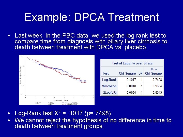
Example: DPCA Treatment • Last week, in the PBC data, we used the log rank test to compare time from diagnosis with biliary liver cirrhosis to death between treatment with DPCA vs. placebo. • Log-Rank test X 2 =. 1017 (p=. 7498) • We cannot reject the hypothesis of no difference in time to death between treatment groups.

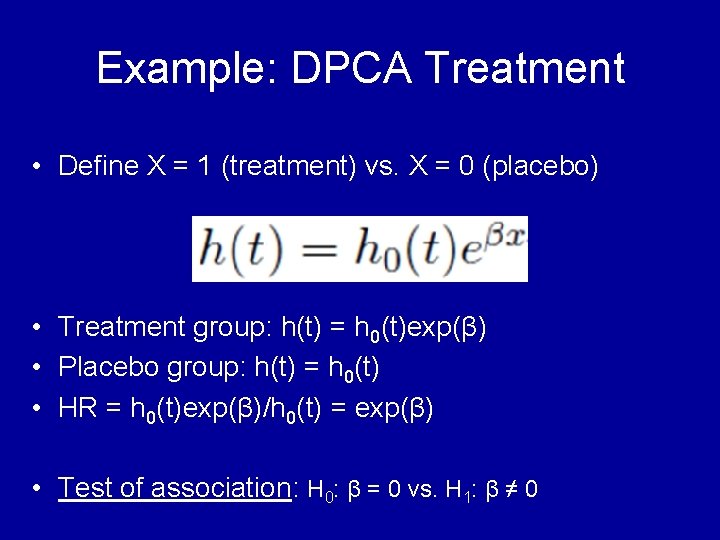
Example: DPCA Treatment • Define X = 1 (treatment) vs. X = 0 (placebo) • Treatment group: h(t) = h 0(t)exp(β) • Placebo group: h(t) = h 0(t) • HR = h 0(t)exp(β)/h 0(t) = exp(β) • Test of association: H 0: β = 0 vs. H 1: β ≠ 0

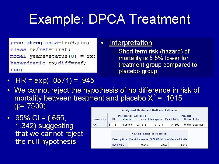
Example: DPCA Treatment • Interpretation: – Short term risk (hazard) of mortality is 5. 5% lower for treatment group compared to placebo group. • HR = exp(-. 0571) =. 945 • We cannot reject the hypothesis of no difference in risk of mortality between treatment and placebo X 2 =. 1015 (p=. 7500) • 95% CI = (. 665, 1. 342) suggesting that we cannot reject the null hypothesis.

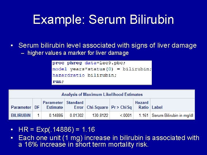
Example: Serum Bilirubin • Serum bilirubin level associated with signs of liver damage – higher values a marker for liver damage • HR = Exp(. 14886) = 1. 16 • Each one unit (1 mg) increase in bilirubin is associated with a 16% increase in short term mortality risk.

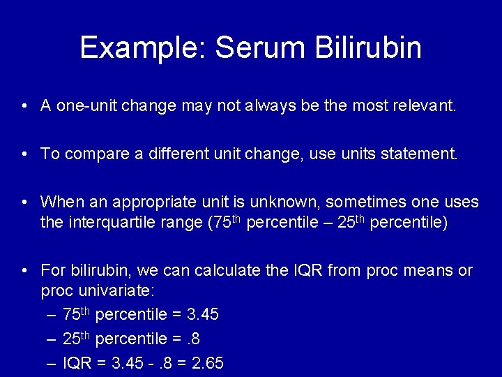
Example: Serum Bilirubin • A one-unit change may not always be the most relevant. • To compare a different unit change, use units statement. • When an appropriate unit is unknown, sometimes one uses the interquartile range (75 th percentile – 25 th percentile) • For bilirubin, we can calculate the IQR from proc means or proc univariate: – 75 th percentile = 3. 45 – 25 th percentile =. 8 – IQR = 3. 45 -. 8 = 2. 65

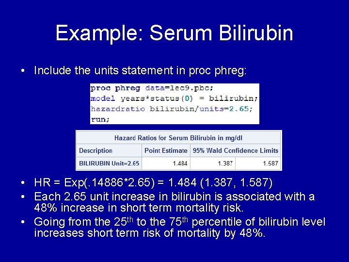
Example: Serum Bilirubin • Include the units statement in proc phreg: • HR = Exp(. 14886*2. 65) = 1. 484 (1. 387, 1. 587) • Each 2. 65 unit increase in bilirubin is associated with a 48% increase in short term mortality risk. • Going from the 25 th to the 75 th percentile of bilirubin level increases short term risk of mortality by 48%.

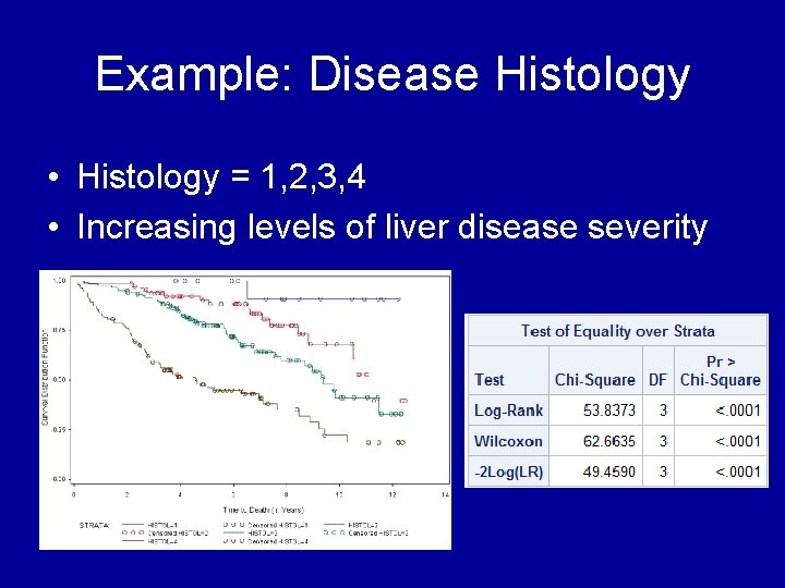
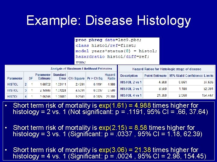
Example: Disease Histology • Histology = 1, 2, 3, 4 • Increasing levels of liver disease severity

Example: Disease Histology • Short term risk of mortality is exp(1. 61) = 4. 988 times higher for histology = 2 vs. 1 (Not significant: p =. 1191, 95% CI =. 66, 37. 64) • Short term risk of mortality is exp(2. 15) = 8. 58 times higher for histology = 3 vs. 1 (Significant: p =. 0337 , 95% CI = 1. 18, 62. 39) • Short term risk of mortality is exp(3. 06) = 21. 38 times higher for histology = 4 vs. 1 (Significant: p =. 0024 , 95% CI = 2. 96, 154. 45)

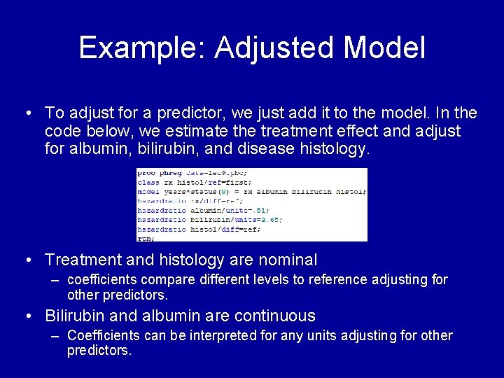
Example: Adjusted Model • To adjust for a predictor, we just add it to the model. In the code below, we estimate the treatment effect and adjust for albumin, bilirubin, and disease histology. • Treatment and histology are nominal – coefficients compare different levels to reference adjusting for other predictors. • Bilirubin and albumin are continuous – Coefficients can be interpreted for any units adjusting for other predictors.

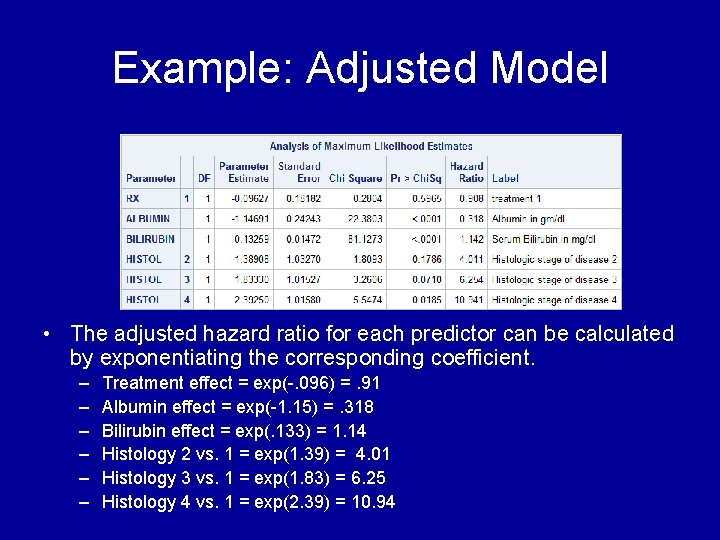
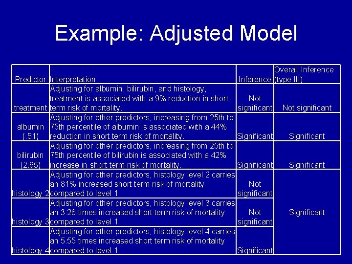
Example: Adjusted Model • The adjusted hazard ratio for each predictor can be calculated by exponentiating the corresponding coefficient. – – – Treatment effect = exp(-. 096) =. 91 Albumin effect = exp(-1. 15) =. 318 Bilirubin effect = exp(. 133) = 1. 14 Histology 2 vs. 1 = exp(1. 39) = 4. 01 Histology 3 vs. 1 = exp(1. 83) = 6. 25 Histology 4 vs. 1 = exp(2. 39) = 10. 94

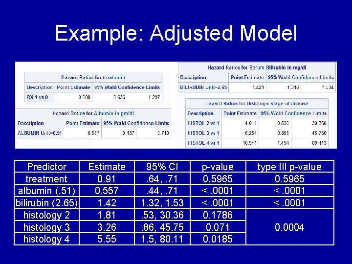
Example: Adjusted Model Predictor treatment albumin (. 51) bilirubin (2. 65) histology 2 histology 3 histology 4 Estimate 0. 91 0. 557 1. 42 1. 81 3. 26 5. 55 95% CI. 64, . 71. 44, . 71 1. 32, 1. 53, 30. 36. 86, 45. 75 1. 5, 80. 11 p-value 0. 5965 <. 0001 0. 1786 0. 071 0. 0185 type III p-value 0. 5965 <. 0001 0. 0004

Example: Adjusted Model Overall Inference (type III) Predictor Interpretation Adjusting for albumin, bilirubin, and histology, treatment is associated with a 9% reduction in short Not treatment term risk of mortality. significant Adjusting for other predictors, increasing from 25 th to albumin 75 th percentile of albumin is associated with a 44% (. 51) reduction in short term risk of mortality. Significant Adjusting for other predictors, increasing from 25 th to bilirubin 75 th percentile of bilirubin is associated with a 42% (2. 65) increase in short term risk of mortality. Significant Adjusting for other predictors, histology level 2 carries an 81% increased short term risk of mortality Not histology 2 compared to level 1 significant Adjusting for other predictors, histology level 3 carries an 3. 26 times increased short term risk of mortality Not histology 3 compared to level 1 significant Adjusting for other predictors, histology level 4 carries an 5. 55 times increased short term risk of mortality histology 4 compared to level 1 Significant Not significant Significant

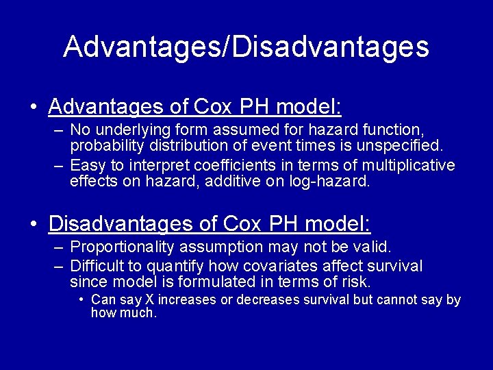
Advantages/Disadvantages • Advantages of Cox PH model: – No underlying form assumed for hazard function, probability distribution of event times is unspecified. – Easy to interpret coefficients in terms of multiplicative effects on hazard, additive on log-hazard. • Disadvantages of Cox PH model: – Proportionality assumption may not be valid. – Difficult to quantify how covariates affect survival since model is formulated in terms of risk. • Can say X increases or decreases survival but cannot say by how much.

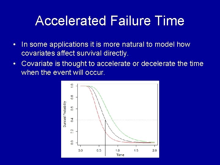
Accelerated Failure Time • In some applications it is more natural to model how covariates affect survival directly. • Covariate is thought to accelerate or decelerate the time when the event will occur.

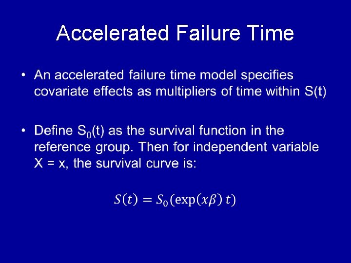
Accelerated Failure Time •

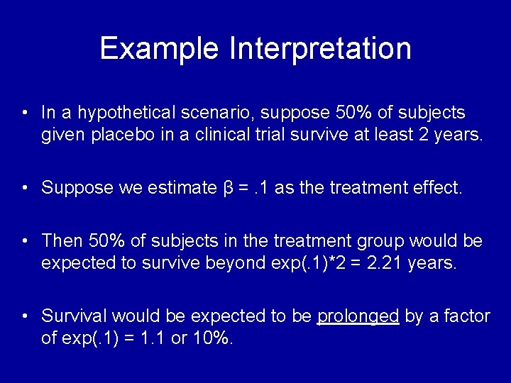
Example Interpretation • In a hypothetical scenario, suppose 50% of subjects given placebo in a clinical trial survive at least 2 years. • Suppose we estimate β =. 1 as the treatment effect. • Then 50% of subjects in the treatment group would be expected to survive beyond exp(. 1)*2 = 2. 21 years. • Survival would be expected to be prolonged by a factor of exp(. 1) = 1. 1 or 10%.

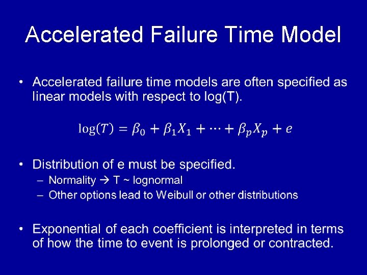
Accelerated Failure Time Model •

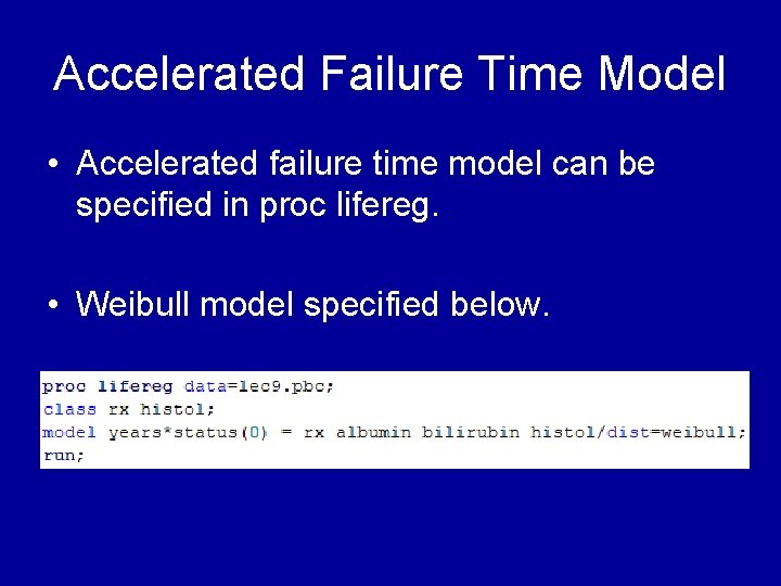
Accelerated Failure Time Model • Accelerated failure time model can be specified in proc lifereg. • Weibull model specified below.

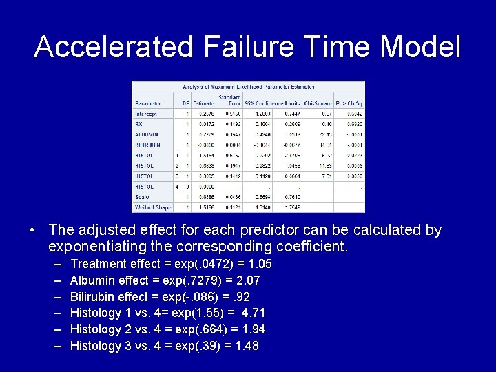
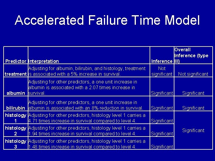
Accelerated Failure Time Model • The adjusted effect for each predictor can be calculated by exponentiating the corresponding coefficient. – – – Treatment effect = exp(. 0472) = 1. 05 Albumin effect = exp(. 7279) = 2. 07 Bilirubin effect = exp(-. 086) =. 92 Histology 1 vs. 4= exp(1. 55) = 4. 71 Histology 2 vs. 4 = exp(. 664) = 1. 94 Histology 3 vs. 4 = exp(. 39) = 1. 48

Accelerated Failure Time Model Predictor Interpretation Overall Inference (type Inference III) Adjusting for albumin, bilirubin, and histology, treatment Not significant treatment is associated with a 5% increase in survival. Not significant Adjusting for other predictors, a one unit increase in albumin is associated with a 2. 07 times increase in albumin survival. Significant Adjusting for other predictors, a one unit increase in bilirubin albumin is associated with an 8% reduction in survival. Significant histology Adjusting for other predictors, histology level 1 carries a 1 4. 71 times increase in survival compared to level 4. Significant histology Adjusting for other predictors, histology level 1 carries a 2 1. 94 times increase in survival compared to level 4. Significant histology Adjusting for other predictors, histology level 1 carries a 3 1. 48 times increase in survival compared to level 4. Significant

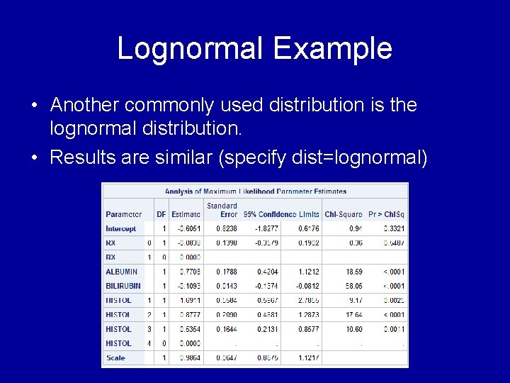
Lognormal Example • Another commonly used distribution is the lognormal distribution. • Results are similar (specify dist=lognormal)