Lecture 8 Principal Component Analysis CSE 6367 Computer

Lecture 8 Principal Component Analysis CSE 6367 – Computer Vision Spring 2010 Vassilis Athitsos University of Texas at Arlington

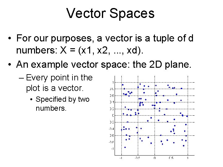
Vector Spaces • For our purposes, a vector is a tuple of d numbers: X = (x 1, x 2, . . . , xd). • An example vector space: the 2 D plane. – Every point in the plot is a vector. • Specified by two numbers.

Images are Vectors • An M-row x N-column image is a vector of dimensionality. . .

Images are Vectors • An M-row x N-column image is a vector of dimensionality. – M*N if the image is grayscale. – M*N*3 if the image is in color.

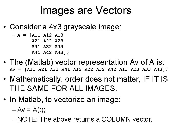
Images are Vectors • Consider a 4 x 3 grayscale image: – A = [A 11 A 21 A 31 A 41 A 12 A 22 A 32 A 42 A 13 A 23 A 33 A 43]; • The (Matlab) vector representation Av of A is: Av = [A 11 A 21 A 31 A 41 A 12 A 22 A 32 A 42 A 13 A 23 A 33 A 43]; • Mathematically, order does not matter, IF IT IS THE SAME FOR ALL IMAGES. • In Matlab, to vectorize an image: – Av = A(: ); – NOTE: The above returns a COLUMN vector.

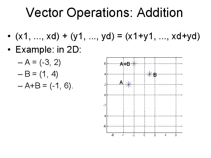
Vector Operations: Addition • (x 1, . . . , xd) + (y 1, . . . , yd) = (x 1+y 1, . . . , xd+yd) • Example: in 2 D: – A = (-3, 2) – B = (1, 4) – A+B = (-1, 6). A+B B A

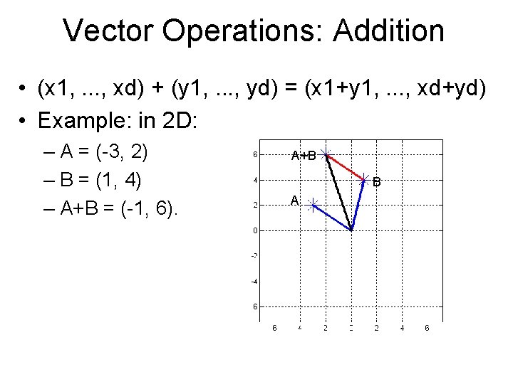
Vector Operations: Addition • (x 1, . . . , xd) + (y 1, . . . , yd) = (x 1+y 1, . . . , xd+yd) • Example: in 2 D: – A = (-3, 2) – B = (1, 4) – A+B = (-1, 6). A+B B A

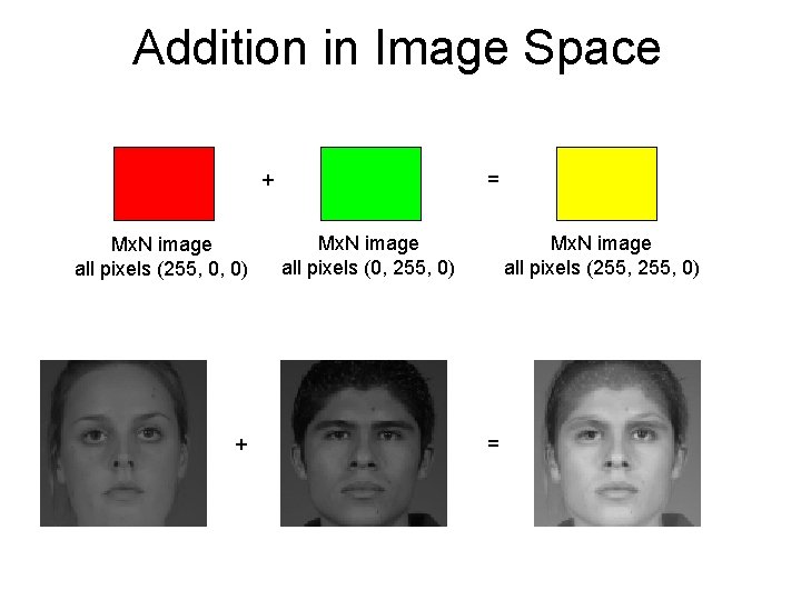
Addition in Image Space = + Mx. N image all pixels (255, 0, 0) + Mx. N image all pixels (0, 255, 0) Mx. N image all pixels (255, 0) =

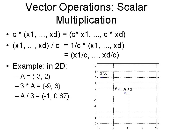
Vector Operations: Scalar Multiplication • c * (x 1, . . . , xd) = (c* x 1, . . . , c * xd) • (x 1, . . . , xd) / c = 1/c * (x 1, . . . , xd) = (x 1/c, . . . , xd/c) • Example: in 2 D: – A = (-3, 2) – 3 * A = (-9, 6) – A / 3 = (-1, 0. 67). 3*A A A/3

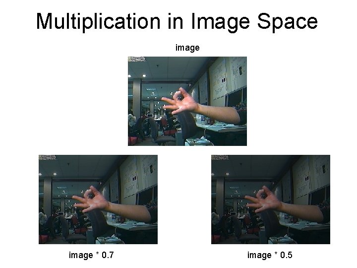
Multiplication in Image Space image * 0. 7 image * 0. 5

Operations in Image Space • Note: with addition and multiplication we can easily generate images with values outside the [0, 255] range. – These operations are perfectly legal. – However, we cannot visualize the results directly. • Must convert back to [0 255] range to visualize.

Linear Combinations • Example: c 1 * v 1 + c 2 * v 2 + c 3 * v 3 – c 1, c 2, c 3: real numbers. – v 1, v 2, v 3: vectors – result:

Linear Combinations • Example: c 1 * v 1 + c 2 * v 2 + c 3 * v 3 – c 1, c 2, c 3: real numbers. – v 1, v 2, v 3: vectors – result: vector.

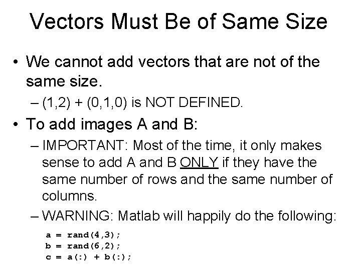
Vectors Must Be of Same Size • We cannot add vectors that are not of the same size. – (1, 2) + (0, 1, 0) is NOT DEFINED. • To add images A and B: – IMPORTANT: Most of the time, it only makes sense to add A and B ONLY if they have the same number of rows and the same number of columns. – WARNING: Matlab will happily do the following: a = rand(4, 3); b = rand(6, 2); c = a(: ) + b(: );

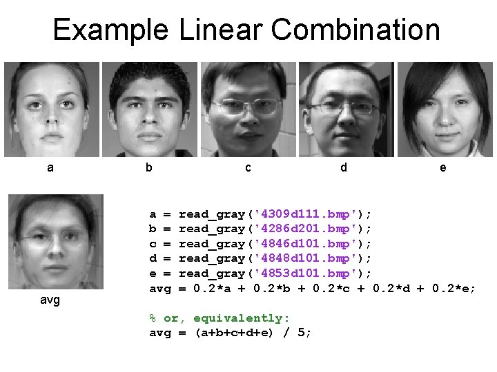
Example Linear Combination a avg b a = b = c = d = e = avg c d e read_gray('4309 d 111. bmp'); read_gray('4286 d 201. bmp'); read_gray('4846 d 101. bmp'); read_gray('4848 d 101. bmp'); read_gray('4853 d 101. bmp'); = 0. 2*a + 0. 2*b + 0. 2*c + 0. 2*d + 0. 2*e; % or, equivalently: avg = (a+b+c+d+e) / 5;

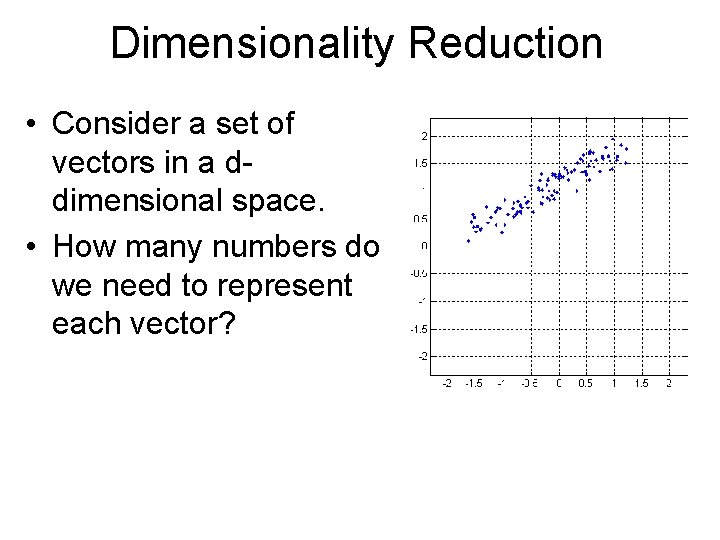
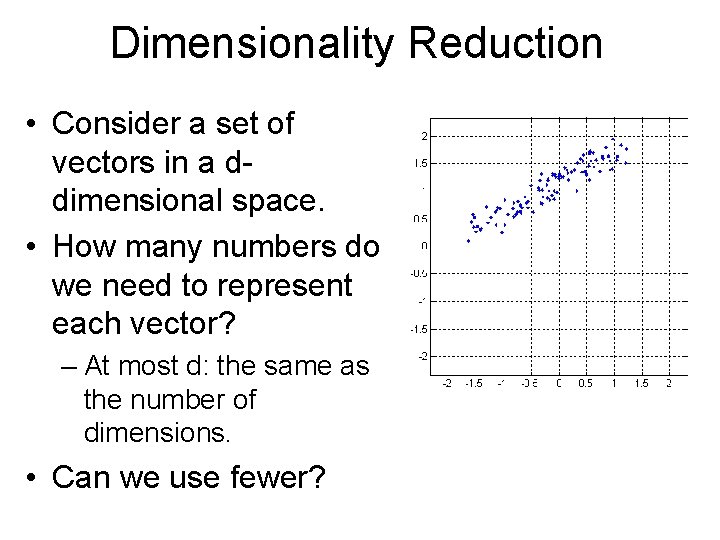
Dimensionality Reduction • Consider a set of vectors in a ddimensional space. • How many numbers do we need to represent each vector?

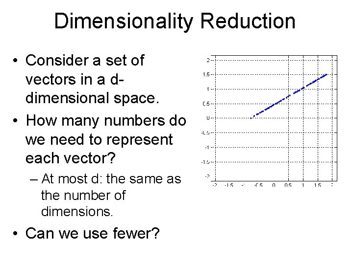
Dimensionality Reduction • Consider a set of vectors in a ddimensional space. • How many numbers do we need to represent each vector? – At most d: the same as the number of dimensions. • Can we use fewer?

Dimensionality Reduction • Consider a set of vectors in a ddimensional space. • How many numbers do we need to represent each vector? – At most d: the same as the number of dimensions. • Can we use fewer?

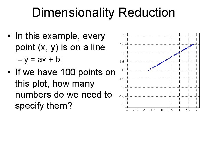
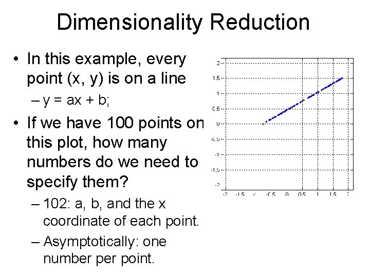
Dimensionality Reduction • In this example, every point (x, y) is on a line – y = ax + b; • If we have 100 points on this plot, how many numbers do we need to specify them?

Dimensionality Reduction • In this example, every point (x, y) is on a line – y = ax + b; • If we have 100 points on this plot, how many numbers do we need to specify them? – 102: a, b, and the x coordinate of each point. – Asymptotically: one number point.

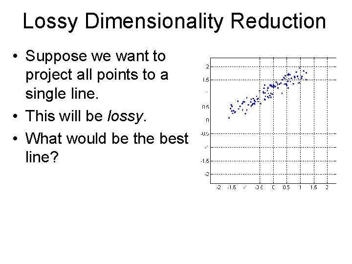
Lossy Dimensionality Reduction • Suppose we want to project all points to a single line. • This will be lossy. • What would be the best line?

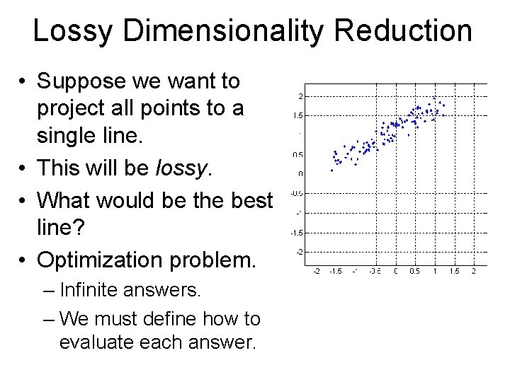
Lossy Dimensionality Reduction • Suppose we want to project all points to a single line. • This will be lossy. • What would be the best line? • Optimization problem. – Infinite answers. – We must define how to evaluate each answer.

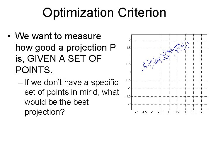
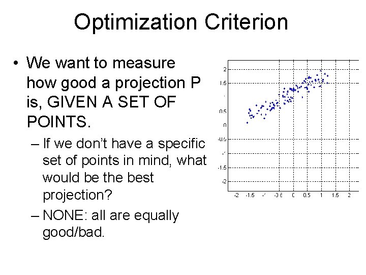
Optimization Criterion • We want to measure how good a projection P is, GIVEN A SET OF POINTS. – If we don’t have a specific set of points in mind, what would be the best projection?

Optimization Criterion • We want to measure how good a projection P is, GIVEN A SET OF POINTS. – If we don’t have a specific set of points in mind, what would be the best projection? – NONE: all are equally good/bad.

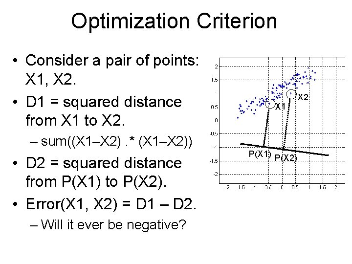
Optimization Criterion • Consider a pair of points: X 1, X 2. • D 1 = squared distance from X 1 to X 2. X 1 – sum((X 1–X 2). * (X 1–X 2)) • D 2 = squared distance from P(X 1) to P(X 2). • Error(X 1, X 2) = D 1 – D 2. – Will it ever be negative? P(X 1) P(X 2) X 2

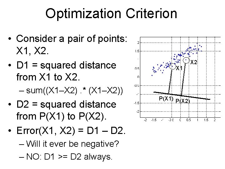
Optimization Criterion • Consider a pair of points: X 1, X 2. • D 1 = squared distance from X 1 to X 2. X 1 – sum((X 1–X 2). * (X 1–X 2)) • D 2 = squared distance from P(X 1) to P(X 2). • Error(X 1, X 2) = D 1 – D 2. – Will it ever be negative? – NO: D 1 >= D 2 always. P(X 1) P(X 2) X 2

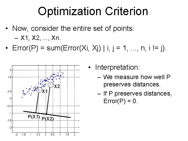
Optimization Criterion • Now, consider the entire set of points: – X 1, X 2, . . . , Xn. • Error(P) = sum(Error(Xi, Xj) | i, j = 1, . . . , n, i != j). • Interpretation: X 1 P(X 1) P(X 2) X 2 – We measure how well P preserves distances. – If P preserves distances, Error(P) = 0.

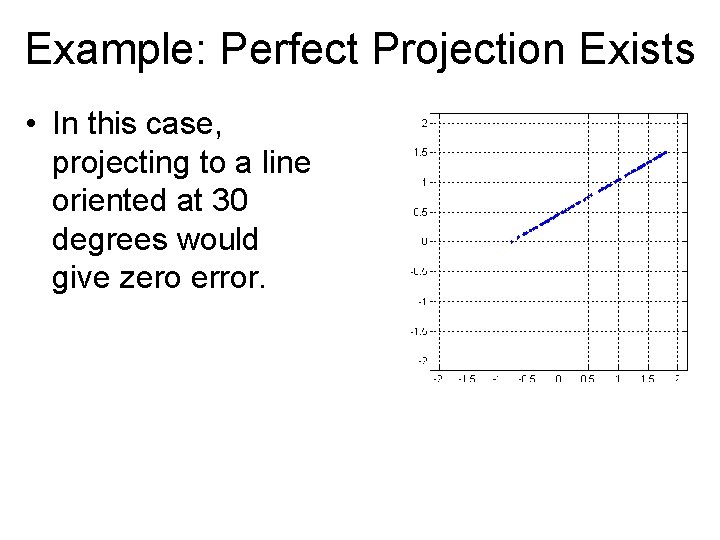
Example: Perfect Projection Exists • In this case, projecting to a line oriented at 30 degrees would give zero error.

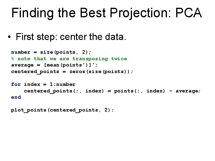
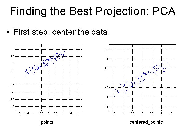
Finding the Best Projection: PCA • First step: center the data. number = size(points, 2); % note that we are transposing twice average = [mean(points')]'; centered_points = zeros(size(points)); for index = 1: number centered_points(: , index) = points(: , index) - average; end plot_points(centered_points, 2);

Finding the Best Projection: PCA • First step: center the data. points centered_points

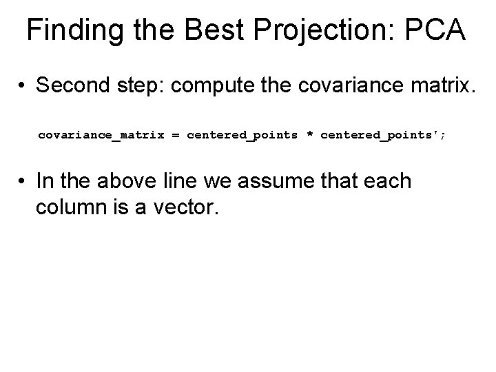
Finding the Best Projection: PCA • Second step: compute the covariance matrix. covariance_matrix = centered_points * centered_points'; • In the above line we assume that each column is a vector.

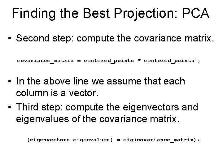
Finding the Best Projection: PCA • Second step: compute the covariance matrix. covariance_matrix = centered_points * centered_points'; • In the above line we assume that each column is a vector. • Third step: compute the eigenvectors and eigenvalues of the covariance matrix. [eigenvectors eigenvalues] = eig(covariance_matrix);

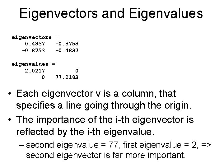
Eigenvectors and Eigenvalues eigenvectors = 0. 4837 -0. 8753 -0. 4837 eigenvalues = 2. 0217 0 0 77. 2183 • Each eigenvector v is a column, that specifies a line going through the origin. • The importance of the i-th eigenvector is reflected by the i-th eigenvalue. – second eigenvalue = 77, first eigenvalue = 2, => second eigenvector is far more important.

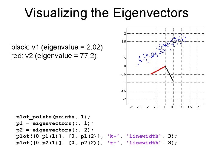
Visualizing the Eigenvectors black: v 1 (eigenvalue = 2. 02) red: v 2 (eigenvalue = 77. 2) plot_points(points, 1); p 1 = eigenvectors(: , 1); p 2 = eigenvectors(: , 2); plot([0 p 1(1)], [0, p 1(2)], 'k-', 'linewidth', 3); plot([0 p 2(1)], [0, p 2(2)], 'r-', 'linewidth', 3);

PCA Code function [average, eigenvectors, eigenvalues] =. . . compute_pca(vectors) number = size(vectors, 2); % note that we are transposing twice average = [mean(vectors')]'; centered_vectors = zeros(size(vectors)); for index = 1: number centered_vectors(: , index) = vectors(: , index) - average; end covariance_matrix = centered_vectors * centered_vectors'; [eigenvectors eigenvalues] = eig( covariance_matrix); % eigenvalues is a matrix, but only the diagonal % matters, so we throw away the rest eigenvalues = diag(eigenvalues); [eigenvalues, indices] = sort(eigenvalues, 'descend'); eigenvectors = eigenvectors(: , indices);

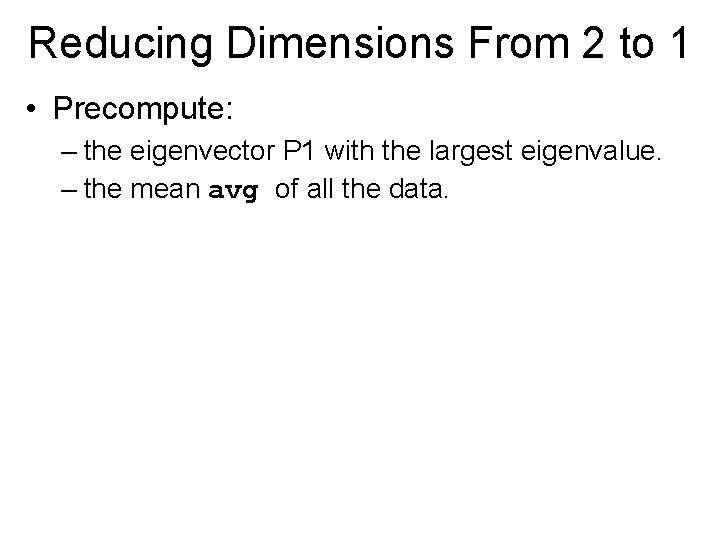
Reducing Dimensions From 2 to 1 • Precompute: – the eigenvector P 1 with the largest eigenvalue. – the mean avg of all the data.

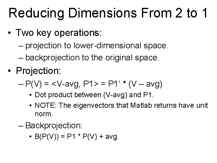
Reducing Dimensions From 2 to 1 • Two key operations: – projection to lower-dimensional space. – backprojection to the original space. • Projection: – P(V) = <V-avg, P 1> = P 1’ * (V – avg) • Dot product between (V-avg) and P 1. • NOTE: The eigenvectors that Matlab returns have unit norm. – Backprojection: • B(P(V)) = P 1 * P(V) + avg.

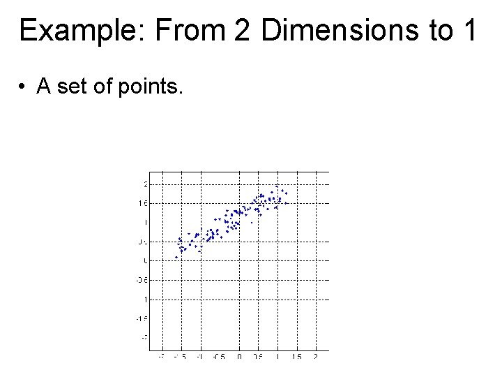
Example: From 2 Dimensions to 1 • A set of points.

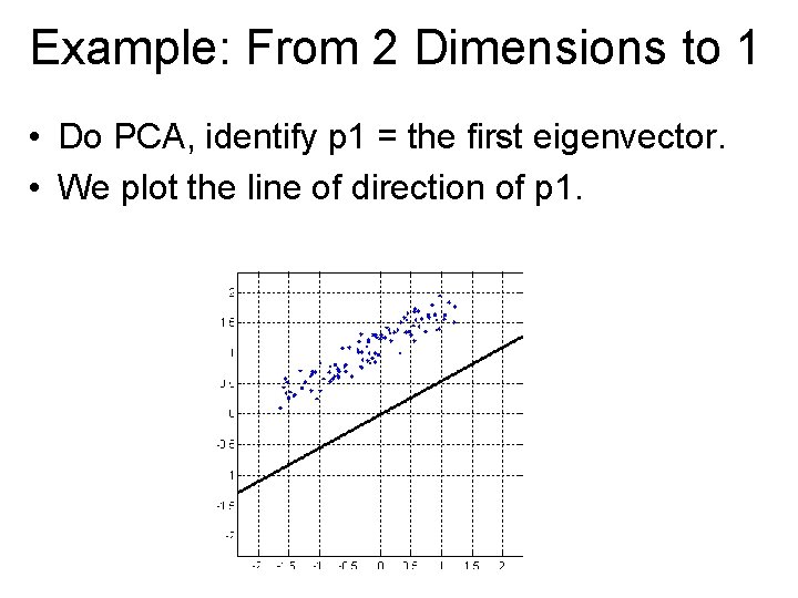
Example: From 2 Dimensions to 1 • Do PCA, identify p 1 = the first eigenvector. • We plot the line of direction of p 1.

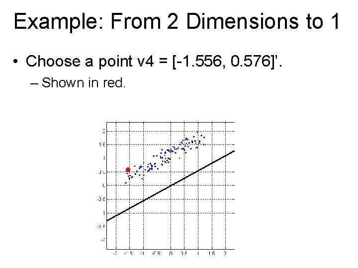
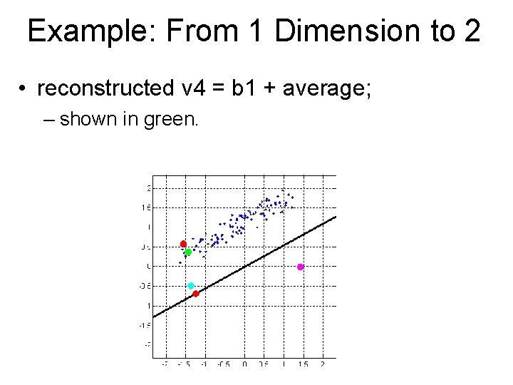
Example: From 2 Dimensions to 1 • Choose a point v 4 = [-1. 556, 0. 576]’. – Shown in red.

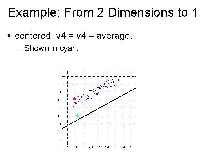
Example: From 2 Dimensions to 1 • centered_v 4 = v 4 – average. – Shown in cyan.

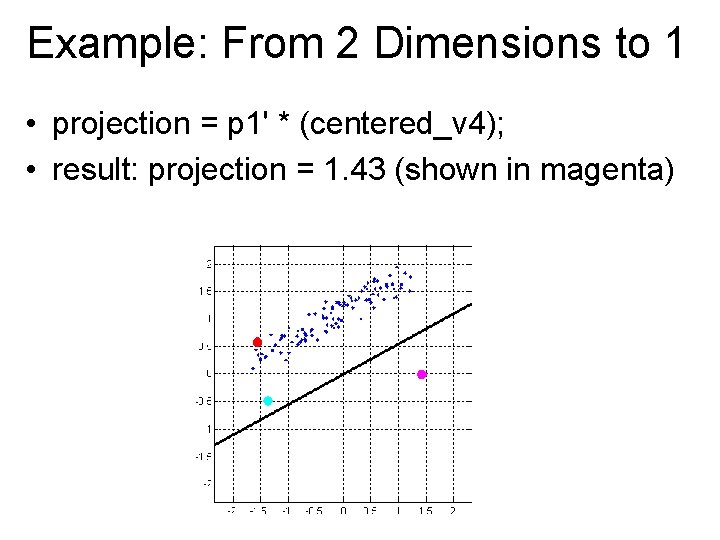
Example: From 2 Dimensions to 1 • projection = p 1' * (centered_v 4); • result: projection = 1. 43 (shown in magenta)

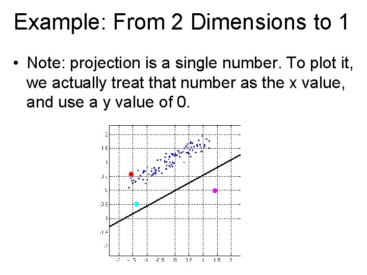
Example: From 2 Dimensions to 1 • Note: projection is a single number. To plot it, we actually treat that number as the x value, and use a y value of 0.

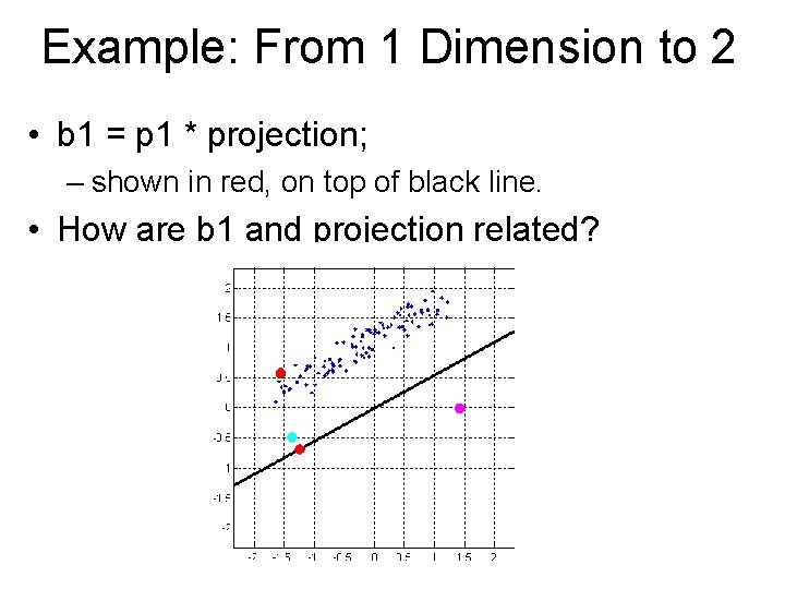
Example: From 1 Dimension to 2 • b 1 = p 1 * projection; – shown in red, on top of black line. • How are b 1 and projection related?

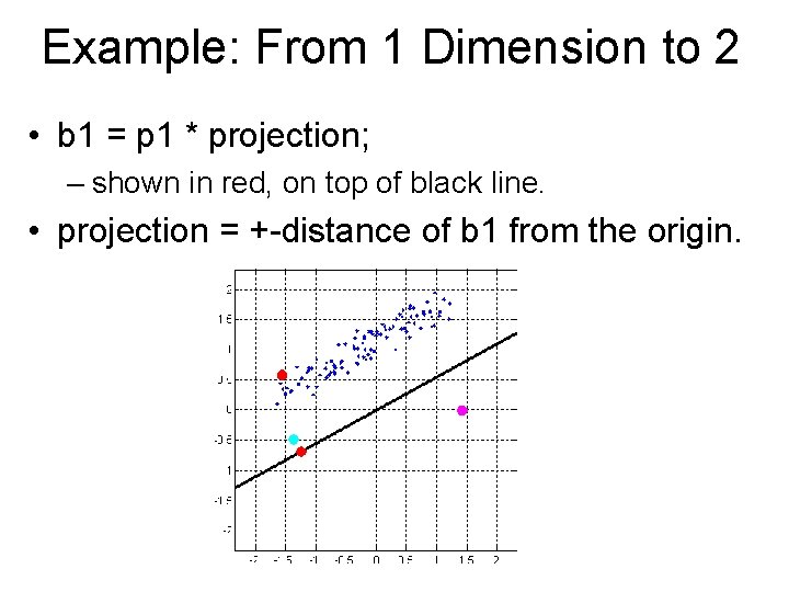
Example: From 1 Dimension to 2 • b 1 = p 1 * projection; – shown in red, on top of black line. • projection = +-distance of b 1 from the origin.

Example: From 1 Dimension to 2 • reconstructed v 4 = b 1 + average; – shown in green.

PCA on Faces • Motivation: If a face is a 31 x 25 window, we need 775 numbers to describe the face. • With PCA, we can approximate face images with much fewer numbers. • Two benefits: – Faster computations. – The amount of loss can be used for face detection.

PCA vs Template Matching • If we use template matching to detect faces, what is the perfect face (easiest to be detected)? • How about PCA?

PCA vs Template Matching • Template matching: – The average face is the only perfect face (after we normalize for brightness and contrast). • As a model, it is not rich enough. • PCA: – There is a space of perfect faces.

Preparing a Dataset • Get a set of face images. – They must be of same size, and aligned, so that eye locations match each other, nose locations match each other, and so on. – Make the mean and std of all faces equal. • Discards variations in intensity and contrast.

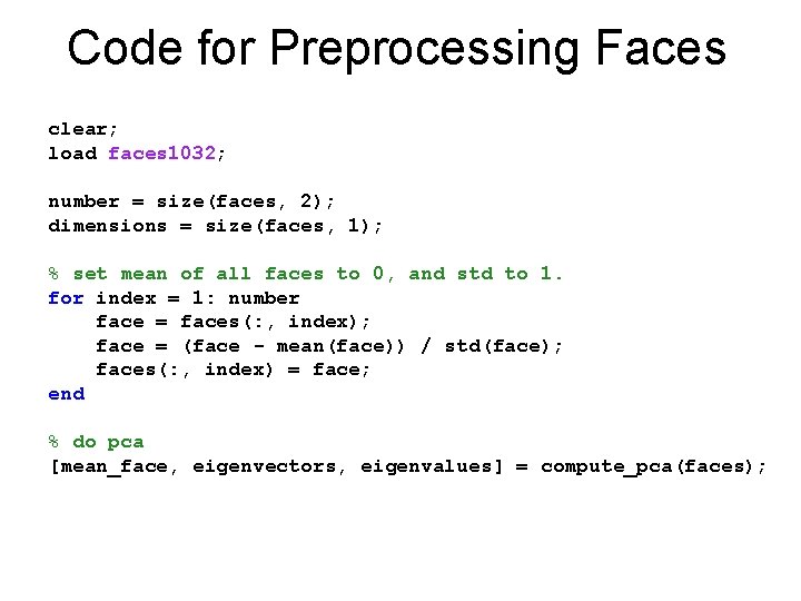
Code for Preprocessing Faces clear; load faces 1032; number = size(faces, 2); dimensions = size(faces, 1); % set mean of all faces to 0, and std to 1. for index = 1: number face = faces(: , index); face = (face - mean(face)) / std(face); faces(: , index) = face; end % do pca [mean_face, eigenvectors, eigenvalues] = compute_pca(faces);

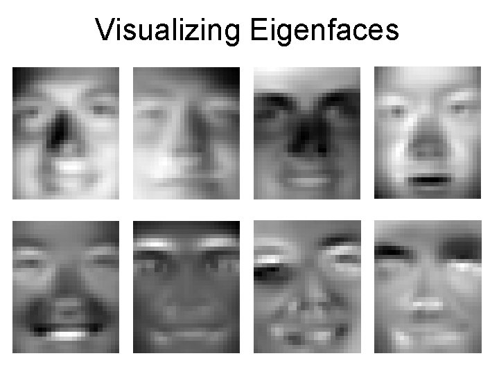
Visualizing Eigenfaces

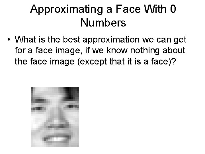
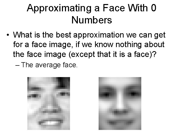
Approximating a Face With 0 Numbers • What is the best approximation we can get for a face image, if we know nothing about the face image (except that it is a face)?

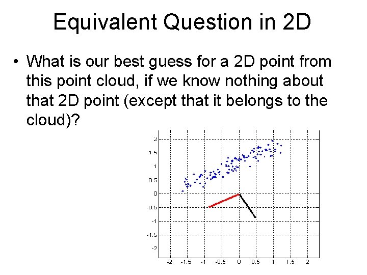
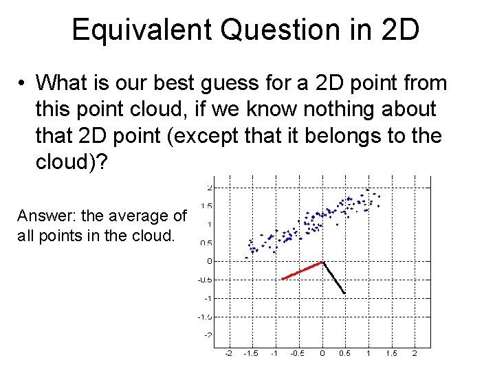
Equivalent Question in 2 D • What is our best guess for a 2 D point from this point cloud, if we know nothing about that 2 D point (except that it belongs to the cloud)?

Equivalent Question in 2 D • What is our best guess for a 2 D point from this point cloud, if we know nothing about that 2 D point (except that it belongs to the cloud)? Answer: the average of all points in the cloud.

Approximating a Face With 0 Numbers • What is the best approximation we can get for a face image, if we know nothing about the face image (except that it is a face)?

Approximating a Face With 0 Numbers • What is the best approximation we can get for a face image, if we know nothing about the face image (except that it is a face)? – The average face.

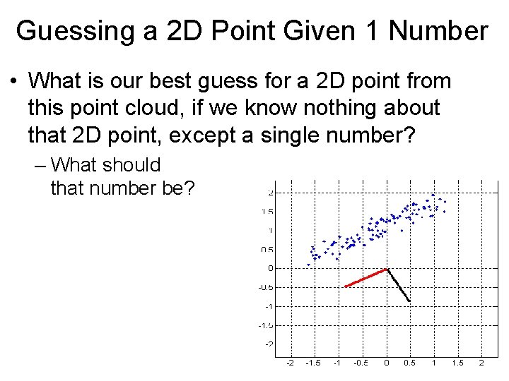
Guessing a 2 D Point Given 1 Number • What is our best guess for a 2 D point from this point cloud, if we know nothing about that 2 D point, except a single number? – What should that number be?

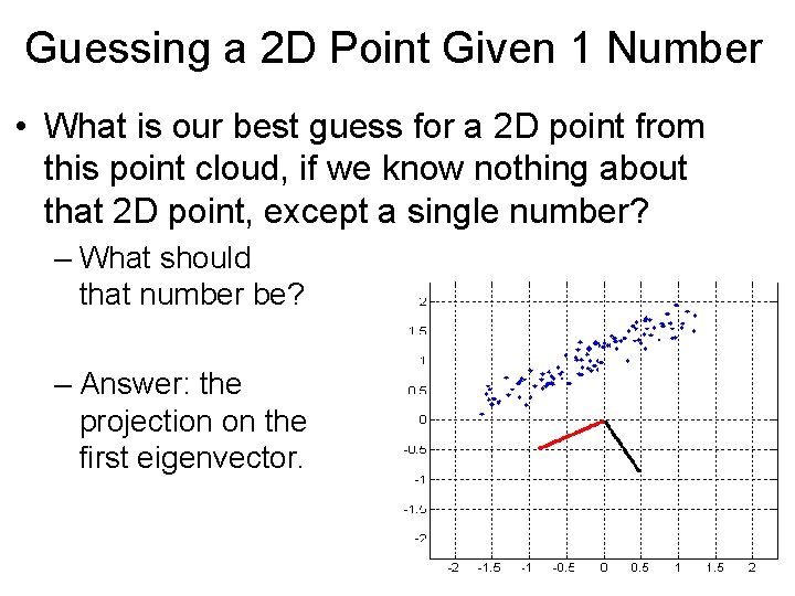
Guessing a 2 D Point Given 1 Number • What is our best guess for a 2 D point from this point cloud, if we know nothing about that 2 D point, except a single number? – What should that number be? – Answer: the projection on the first eigenvector.

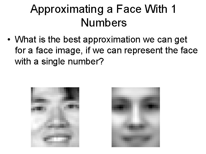
Approximating a Face With 1 Numbers • What is the best approximation we can get for a face image, if we can represent the face with a single number?

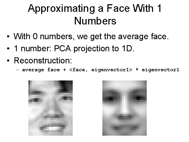
Approximating a Face With 1 Numbers • With 0 numbers, we get the average face. • 1 number: PCA projection to 1 D. • Reconstruction: – average face + <face, eigenvector 1> * eigenvector 1

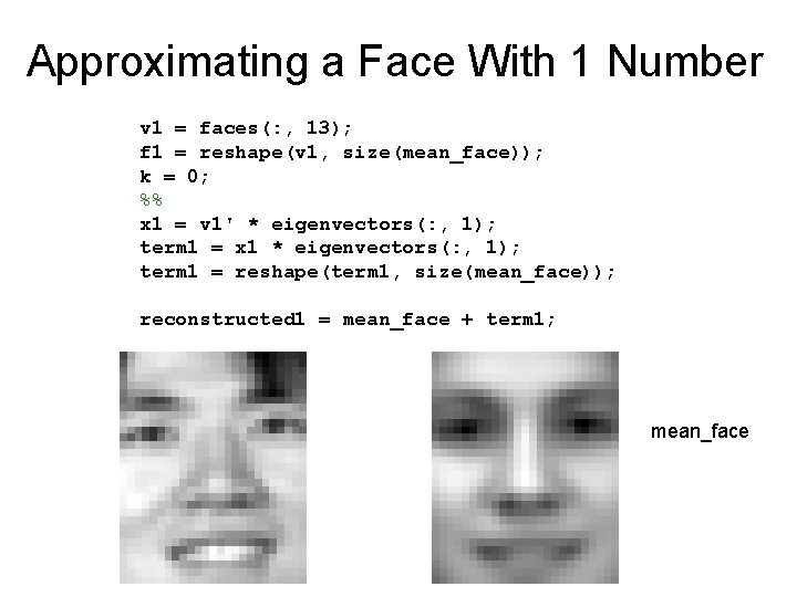
Approximating a Face With 1 Number v 1 = faces(: , 13); f 1 = reshape(v 1, size(mean_face)); k = 0; %% x 1 = v 1' * eigenvectors(: , 1); term 1 = x 1 * eigenvectors(: , 1); term 1 = reshape(term 1, size(mean_face)); reconstructed 1 = mean_face + term 1; mean_face

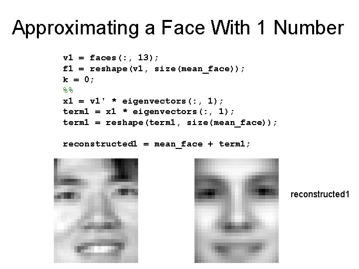
Approximating a Face With 1 Number v 1 = faces(: , 13); f 1 = reshape(v 1, size(mean_face)); k = 0; %% x 1 = v 1' * eigenvectors(: , 1); term 1 = x 1 * eigenvectors(: , 1); term 1 = reshape(term 1, size(mean_face)); reconstructed 1 = mean_face + term 1; reconstructed 1

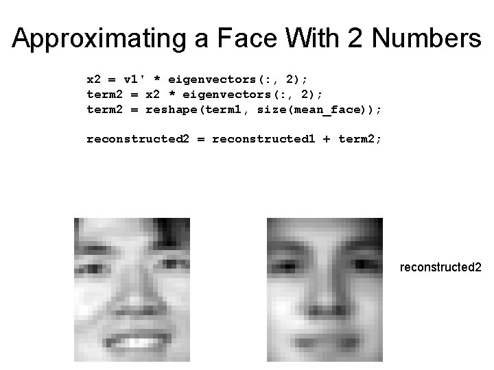
Approximating a Face With 2 Numbers x 2 = v 1' * eigenvectors(: , 2); term 2 = x 2 * eigenvectors(: , 2); term 2 = reshape(term 1, size(mean_face)); reconstructed 2 = reconstructed 1 + term 2; reconstructed 2

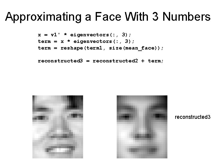
Approximating a Face With 3 Numbers x = v 1' * eigenvectors(: , 3); term = x * eigenvectors(: , 3); term = reshape(term 1, size(mean_face)); reconstructed 3 = reconstructed 2 + term; reconstructed 3

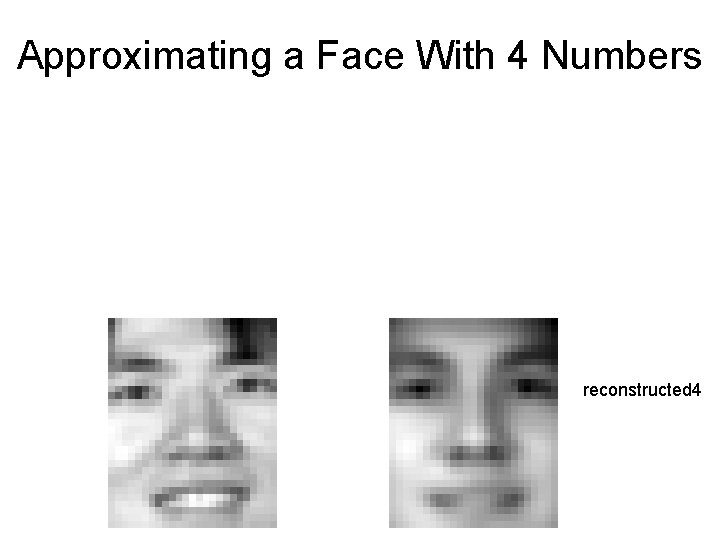
Approximating a Face With 4 Numbers reconstructed 4

Approximating a Face With 5 Numbers reconstructed 5

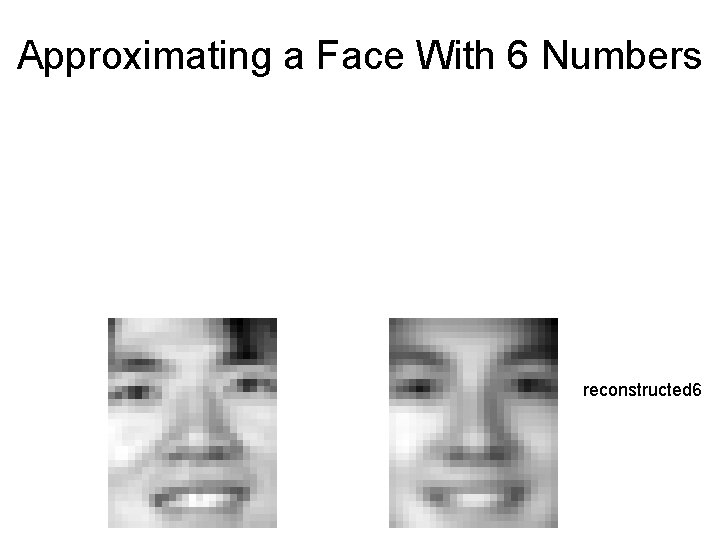
Approximating a Face With 6 Numbers reconstructed 6

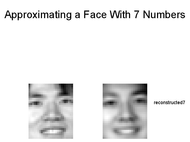
Approximating a Face With 7 Numbers reconstructed 7

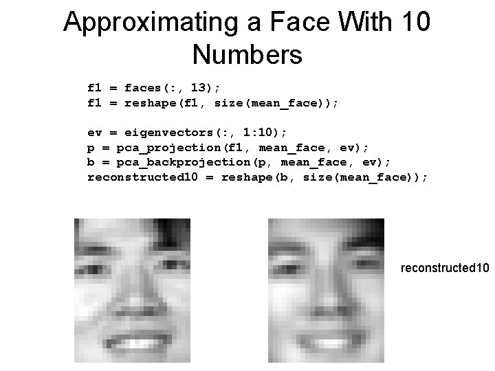
Approximating a Face With 10 Numbers f 1 = faces(: , 13); f 1 = reshape(f 1, size(mean_face)); ev = eigenvectors(: , 1: 10); p = pca_projection(f 1, mean_face, ev); b = pca_backprojection(p, mean_face, ev); reconstructed 10 = reshape(b, size(mean_face)); reconstructed 10

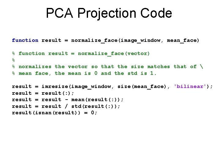
PCA Projection Code function result = normalize_face(image_window, mean_face) % function result = normalize_face(vector) % % normalizes the vector so that the size matches that of % mean face, the mean is 0 and the std is 1. result = imresize(image_window, size(mean_face), 'bilinear'); result = result(: ); result = result - mean(result(: )); result = result / std(result(: )); result(isnan(result)) = 0;

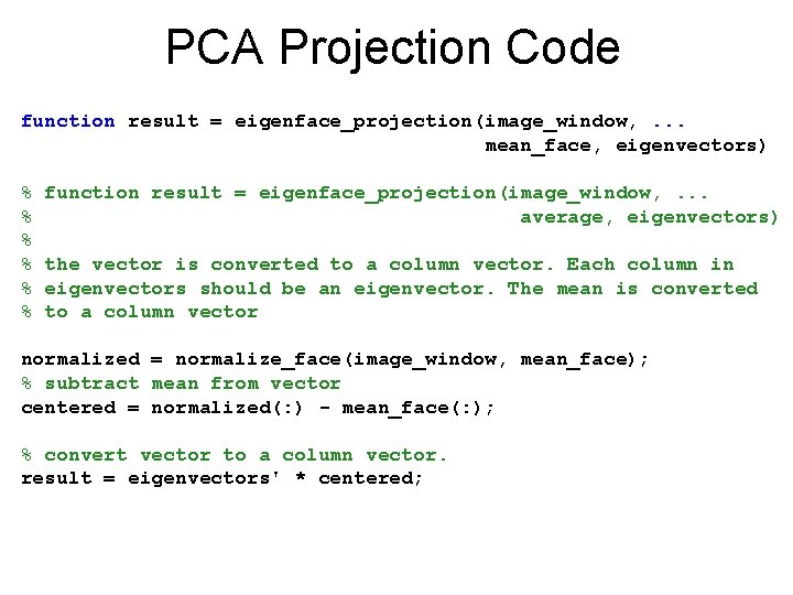
PCA Projection Code function result = eigenface_projection(image_window, . . . mean_face, eigenvectors) % % % function result = eigenface_projection(image_window, . . . average, eigenvectors) the vector is converted to a column vector. Each column in eigenvectors should be an eigenvector. The mean is converted to a column vector normalized = normalize_face(image_window, mean_face); % subtract mean from vector centered = normalized(: ) - mean_face(: ); % convert vector to a column vector. result = eigenvectors' * centered;

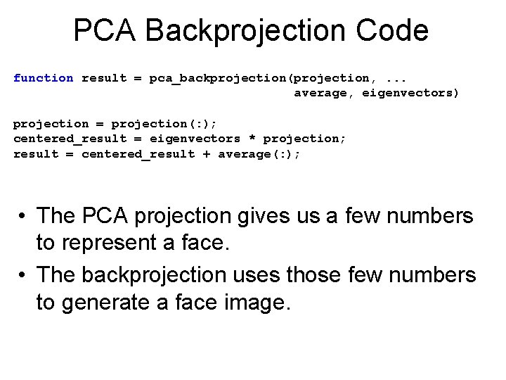
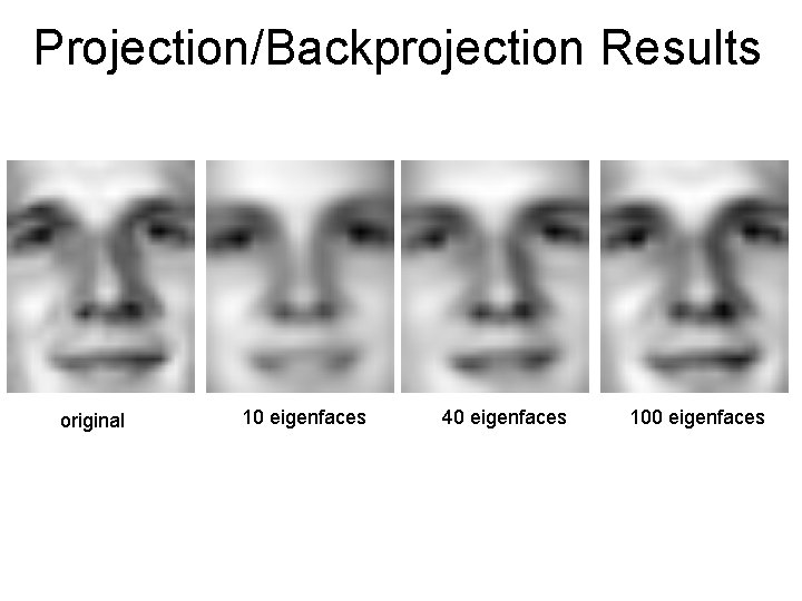
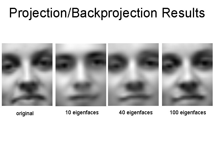
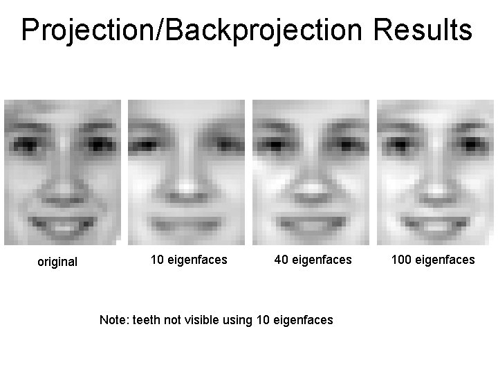
PCA Backprojection Code function result = pca_backprojection(projection, . . . average, eigenvectors) projection = projection(: ); centered_result = eigenvectors * projection; result = centered_result + average(: ); • The PCA projection gives us a few numbers to represent a face. • The backprojection uses those few numbers to generate a face image.

Projection/Backprojection Results original 10 eigenfaces 40 eigenfaces 100 eigenfaces

Projection/Backprojection Results original 10 eigenfaces 40 eigenfaces 100 eigenfaces

Projection/Backprojection Results original 10 eigenfaces 40 eigenfaces Note: teeth not visible using 10 eigenfaces 100 eigenfaces

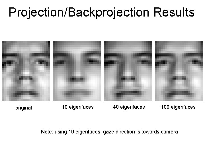
Projection/Backprojection Results original 10 eigenfaces 40 eigenfaces 100 eigenfaces Note: using 10 eigenfaces, gaze direction is towards camera

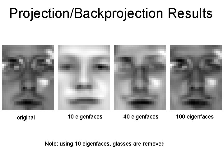
Projection/Backprojection Results original 10 eigenfaces 40 eigenfaces Note: using 10 eigenfaces, glasses are removed 100 eigenfaces

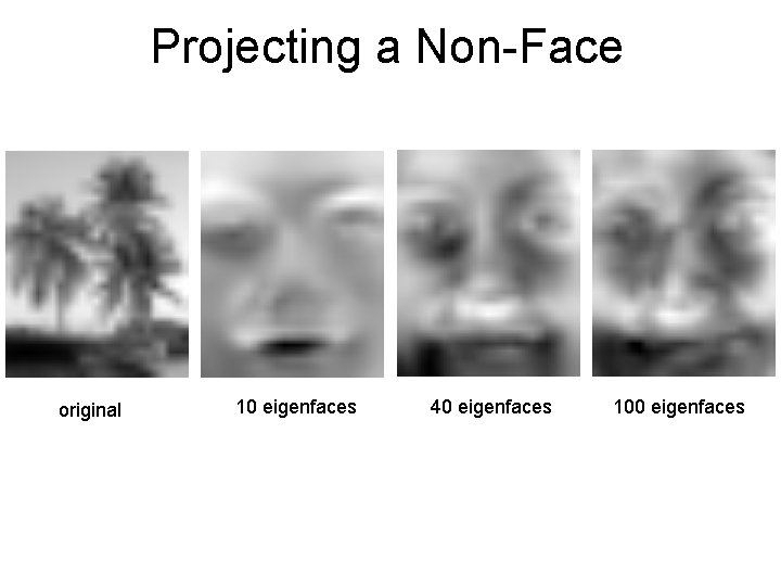
Projecting a Non-Face original 10 eigenfaces 40 eigenfaces 100 eigenfaces

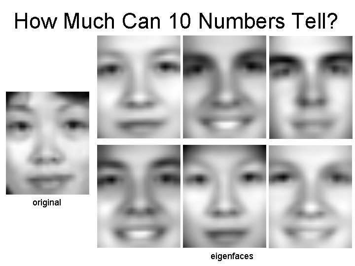
How Much Can 10 Numbers Tell? original eigenfaces