LECTURE 8 FACTOR MODELS Asset Pricing and Portfolio

LECTURE 8 : FACTOR MODELS (Asset Pricing and Portfolio Theory)

Contents The CAPM n Single index model n Arbitrage portfolio. S n Which factors explain asset prices ? n Empirical results n

Introduction n CAPM : Equilibrium model – One factor, where the factor is the excess return on the market. – Based on mean-variance analysis n Stephen Ross (1976) developed alternative model Arbitrage Pricing Theory (APT)

Single Index Model

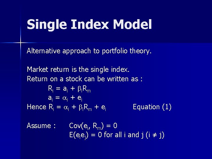
Single Index Model Alternative approach to portfolio theory. Market return is the single index. Return on a stock can be written as : R i = a i + b i. R m a i = a i + ei Hence Ri = ai + bi. Rm + ei Equation (1) Assume : Cov(ei, Rm) = 0 E(eiej) = 0 for all i and j (i ≠ j)

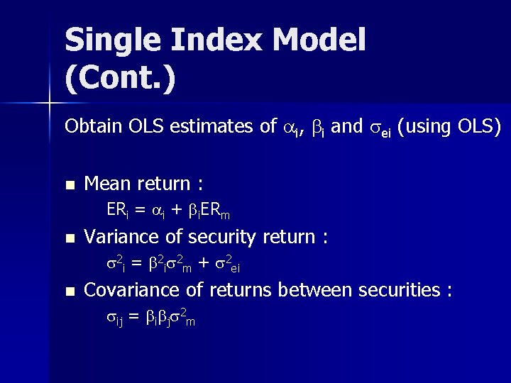
Single Index Model (Cont. ) Obtain OLS estimates of ai, bi and sei (using OLS) n Mean return : ERi = ai + bi. ERm n Variance of security return : s 2 i = b 2 is 2 m + s 2 ei n Covariance of returns between securities : sij = bibjs 2 m

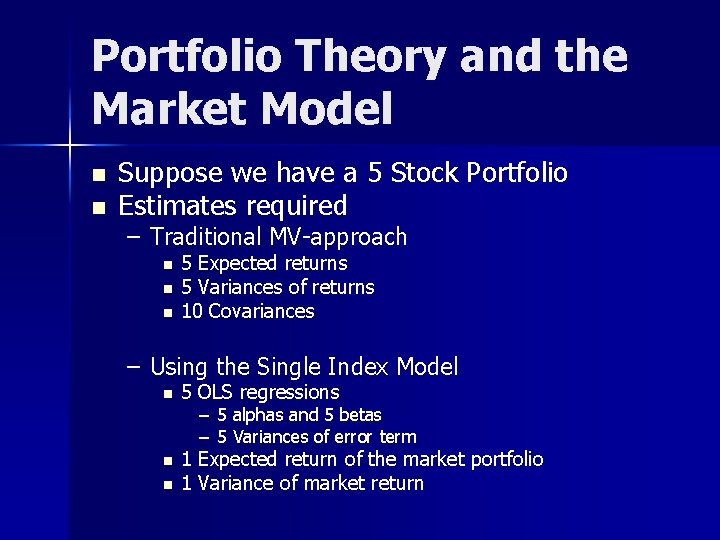
Portfolio Theory and the Market Model n n Suppose we have a 5 Stock Portfolio Estimates required – Traditional MV-approach n n n 5 Expected returns 5 Variances of returns 10 Covariances – Using the Single Index Model n 5 OLS regressions n 1 Expected return of the market portfolio 1 Variance of market return n – 5 alphas and 5 betas – 5 Variances of error term

Factor Models

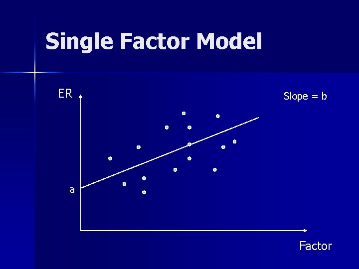
Single Factor Model ER Slope = b a Factor

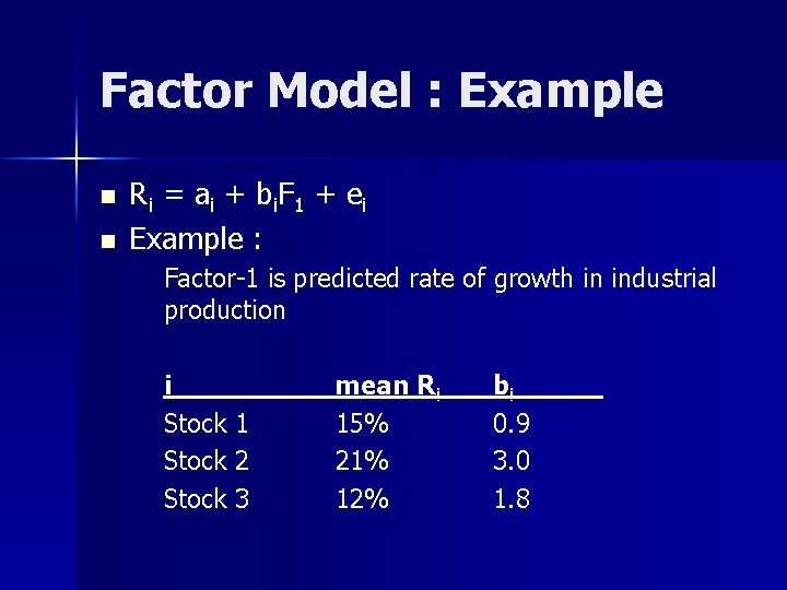
Factor Model : Example n n R i = a i + b i. F 1 + ei Example : Factor-1 is predicted rate of growth in industrial production i Stock 1 Stock 2 Stock 3 mean Ri 15% 21% 12% bi 0. 9 3. 0 1. 8

The APT : Some Thoughts n The Arbitrage Pricing Theory – New and different approach to determine asset prices. – Based on the law of one price : two items that are the same cannot sell at different prices. – Requires fewer assumptions than CAPM – Assumption : each investor, when given the opportunity to increase the return of his portfolio without increasing risk, will do so. n Mechanism for doing so : arbitrage portfolio

An Arbitrage Portfolio

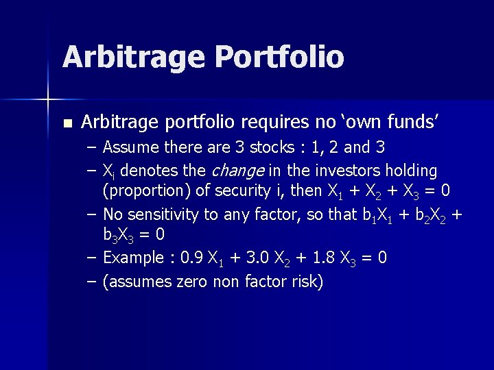
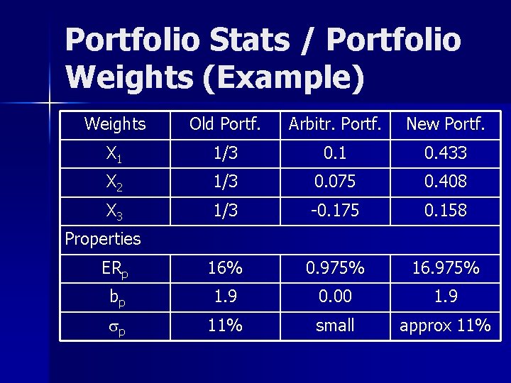
Arbitrage Portfolio n Arbitrage portfolio requires no ‘own funds’ – Assume there are 3 stocks : 1, 2 and 3 – Xi denotes the change in the investors holding (proportion) of security i, then X 1 + X 2 + X 3 = 0 – No sensitivity to any factor, so that b 1 X 1 + b 2 X 2 + b 3 X 3 = 0 – Example : 0. 9 X 1 + 3. 0 X 2 + 1. 8 X 3 = 0 – (assumes zero non factor risk)

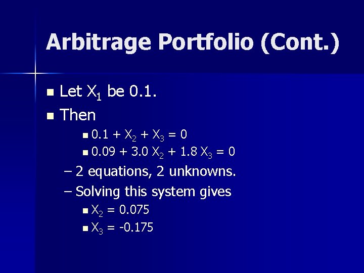
Arbitrage Portfolio (Cont. ) Let X 1 be 0. 1. n Then n n 0. 1 + X 2 + X 3 = 0 n 0. 09 + 3. 0 X 2 + 1. 8 X 3 = 0 – 2 equations, 2 unknowns. – Solving this system gives n X 2 = 0. 075 n X 3 = -0. 175

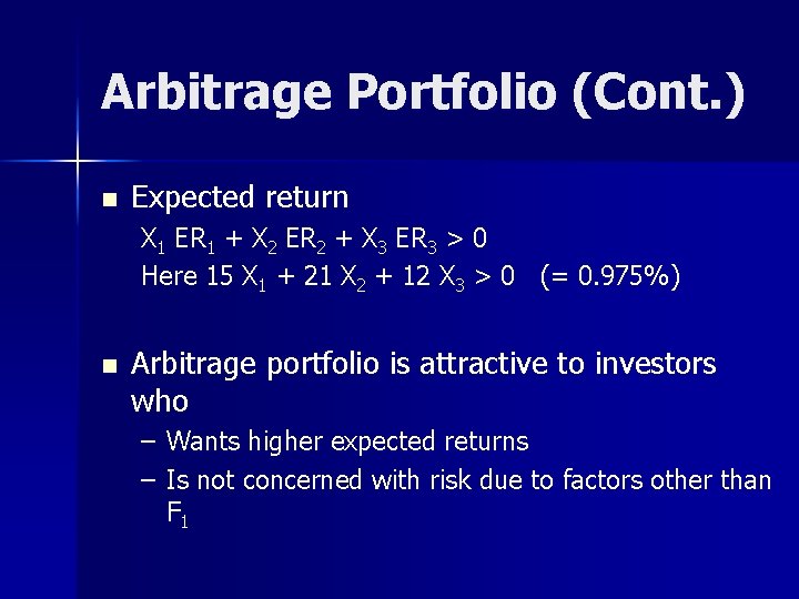
Arbitrage Portfolio (Cont. ) n Expected return X 1 ER 1 + X 2 ER 2 + X 3 ER 3 > 0 Here 15 X 1 + 21 X 2 + 12 X 3 > 0 (= 0. 975%) n Arbitrage portfolio is attractive to investors who – Wants higher expected returns – Is not concerned with risk due to factors other than F 1

Portfolio Stats / Portfolio Weights (Example) Weights Old Portf. Arbitr. Portf. New Portf. X 1 1/3 0. 1 0. 433 X 2 1/3 0. 075 0. 408 X 3 1/3 -0. 175 0. 158 ERp 16% 0. 975% 16. 975% bp 1. 9 0. 00 1. 9 sp 11% small approx 11% Properties

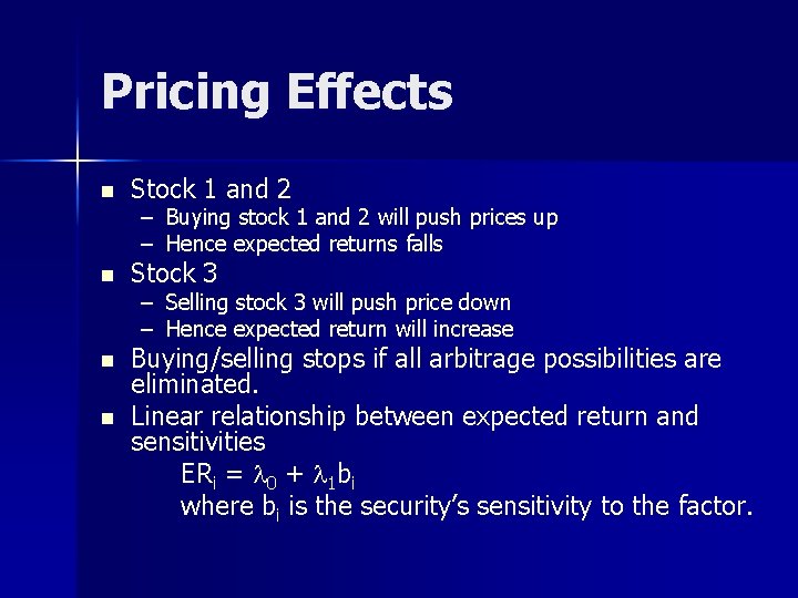
Pricing Effects n Stock 1 and 2 – – Buying stock 1 and 2 will push prices up Hence expected returns falls n Stock 3 n Buying/selling stops if all arbitrage possibilities are eliminated. Linear relationship between expected return and sensitivities ERi = l 0 + l 1 bi where bi is the security’s sensitivity to the factor. n – Selling stock 3 will push price down – Hence expected return will increase

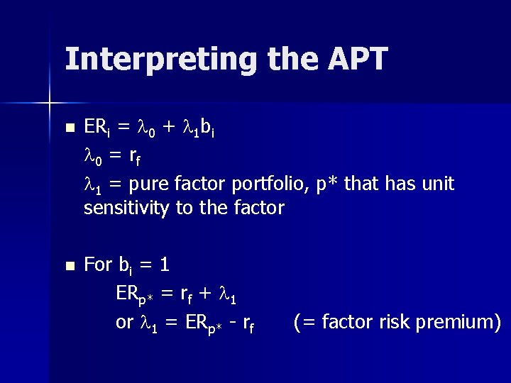
Interpreting the APT n n ERi = l 0 + l 1 bi l 0 = rf l 1 = pure factor portfolio, p* that has unit sensitivity to the factor For bi = 1 ERp* = rf + l 1 or l 1 = ERp* - rf (= factor risk premium)

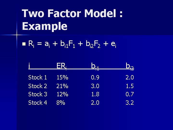
Two Factor Model : Example n Ri = ai + bi 1 F 1 + bi 2 F 2 + ei i ERi bi 1 bi 2 Stock 1 Stock 2 Stock 3 Stock 4 15% 21% 12% 8% 0. 9 3. 0 1. 8 2. 0 1. 5 0. 7 3. 2

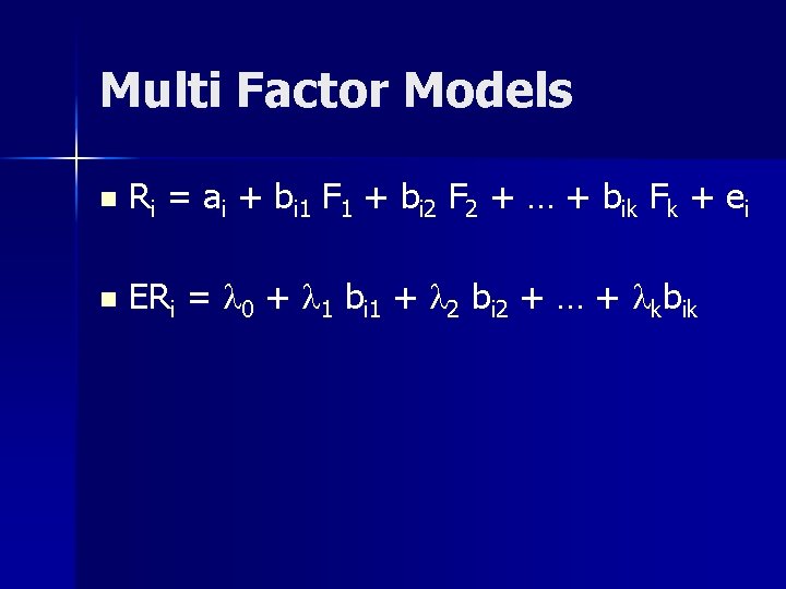
Multi Factor Models n Ri = ai + bi 1 F 1 + bi 2 F 2 + … + bik Fk + ei n ERi = l 0 + l 1 bi 1 + l 2 bi 2 + … + lkbik

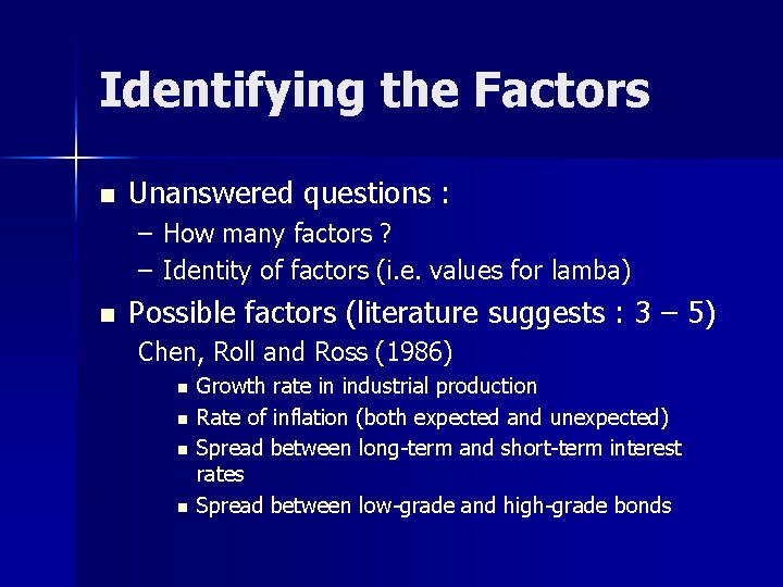
Identifying the Factors n Unanswered questions : – How many factors ? – Identity of factors (i. e. values for lamba) n Possible factors (literature suggests : 3 – 5) Chen, Roll and Ross (1986) n n Growth rate in industrial production Rate of inflation (both expected and unexpected) Spread between long-term and short-term interest rates Spread between low-grade and high-grade bonds

Testing the APT

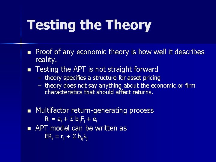
Testing the Theory n n Proof of any economic theory is how well it describes reality. Testing the APT is not straight forward – theory specifies a structure for asset pricing – theory does not say anything about the economic or firm characteristics that should affect returns. n Multifactor return-generating process Ri = ai + S bij. Fj + ei n APT model can be written as ERi = rf + S bijlj

Testing the Theory (Cont. ) bij : are unique to each security and represent an attribute of the security Fj : any I affects more than 1 security (if not all). lj : the extra return required because of a security’s sensitivity to the jth attribute of the security

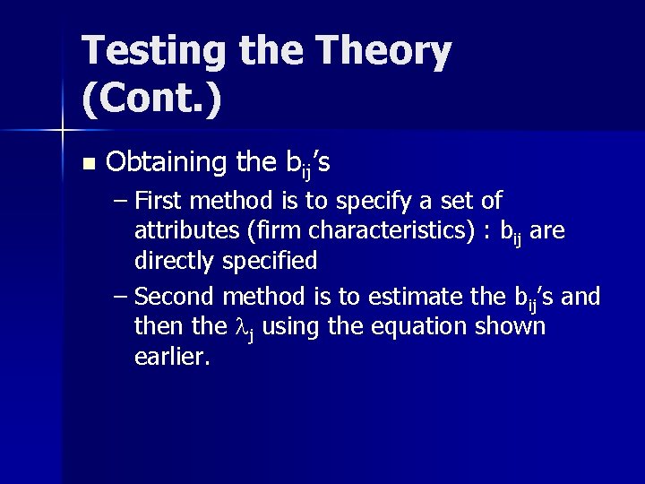
Testing the Theory (Cont. ) n Obtaining the bij’s – First method is to specify a set of attributes (firm characteristics) : bij are directly specified – Second method is to estimate the bij’s and then the lj using the equation shown earlier.

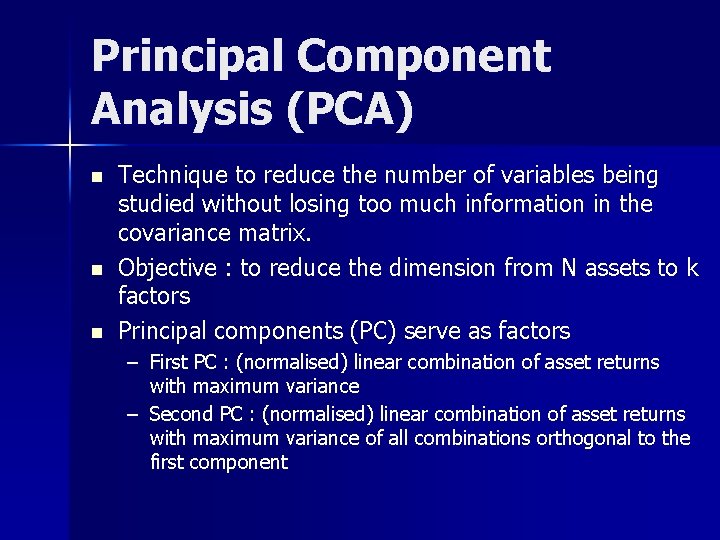
Principal Component Analysis (PCA) n n n Technique to reduce the number of variables being studied without losing too much information in the covariance matrix. Objective : to reduce the dimension from N assets to k factors Principal components (PC) serve as factors – First PC : (normalised) linear combination of asset returns with maximum variance – Second PC : (normalised) linear combination of asset returns with maximum variance of all combinations orthogonal to the first component

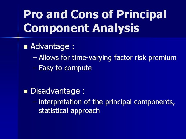
Pro and Cons of Principal Component Analysis n Advantage : – Allows for time-varying factor risk premium – Easy to compute n Disadvantage : – interpretation of the principal components, statistical approach

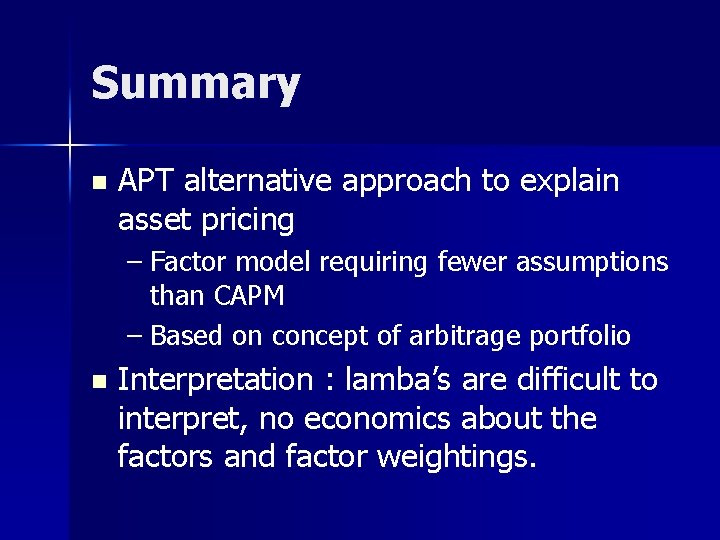
Summary n APT alternative approach to explain asset pricing – Factor model requiring fewer assumptions than CAPM – Based on concept of arbitrage portfolio n Interpretation : lamba’s are difficult to interpret, no economics about the factors and factor weightings.

References Cuthbertson, K. and Nitzsche, D. (2004) ‘Quantitative Financial Economics’, Chapters 7 n Cuthbertson, K. and Nitzsche, D. (2001) ‘Investments : Spot and Derivatives Markets’, Chapter 10. 5 (The Arbitrage Pricing Theory) n

END OF LECTURE