Lecture 8 Applications of Supervised Learning Part II

Lecture 8: Applications of Supervised Learning Part II INFO 1998: Introduction to Machine Learning

Agenda 1. Linear Classifiers 2. Validation: Classification vs Regression 3. Review: Bias-Variance trade-off 4. More Cross-Validation techniques 5. Train-Test Size

Linear Classifiers

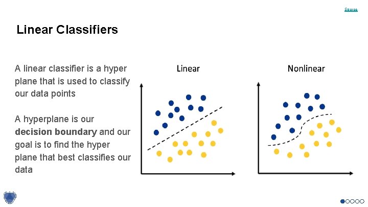
Source Linear Classifiers A linear classifier is a hyper plane that is used to classify our data points A hyperplane is our decision boundary and our goal is to find the hyper plane that best classifies our data

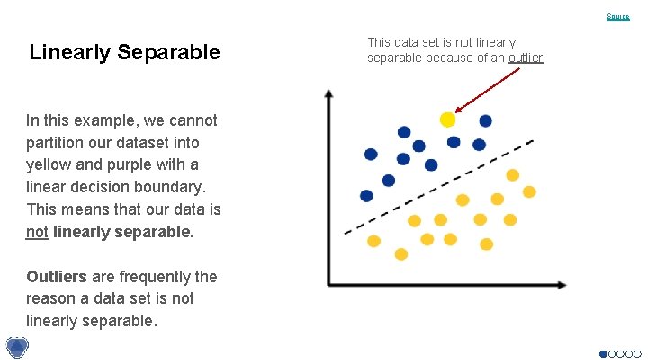
Source Linearly Separable In this example, we cannot partition our dataset into yellow and purple with a linear decision boundary. This means that our data is not linearly separable. Outliers are frequently the reason a data set is not linearly separable. This data set is not linearly separable because of an outlier

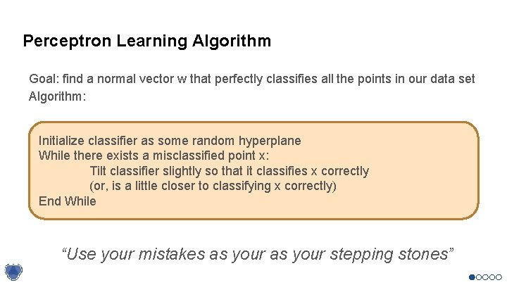
Perceptron Learning Algorithm Goal: find a normal vector w that perfectly classifies all the points in our data set Algorithm: Initialize classifier as some random hyperplane While there exists a misclassified point x: Tilt classifier slightly so that it classifies x correctly (or, is a little closer to classifying x correctly) End While “Use your mistakes as your stepping stones”

Demo

Limitations of Perceptron The training algorithm will never terminate if your training dataset is not linearly separable ☹ Is a great model to understand the intuition behind the training of a linear classifier: iteratively improve classifier by using misclassified points ☺

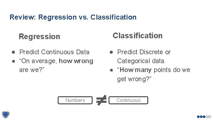
Review: Regression vs. Classification Regression ● Predict Continuous Data ● Predict Discrete or ● “On average, how wrong are we? ” Categorical data ● “How many points do we get wrong? ” Numbers Continuous

Recap: Underfitting, Overfitting, Bias-Variance Tradeoff

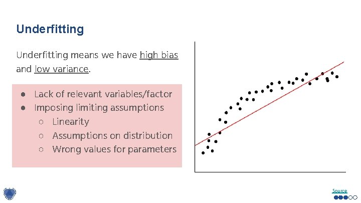
Underfitting means we have high bias and low variance. ● Lack of relevant variables/factor ● Imposing limiting assumptions ○ Linearity ○ Assumptions on distribution ○ Wrong values for parameters Source

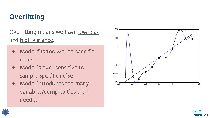
Overfitting means we have low bias and high variance. ● Model fits too well to specific cases ● Model is over-sensitive to sample-specific noise ● Model introduces too many variables/complexities than needed Source

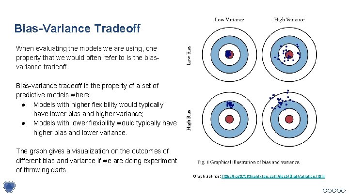
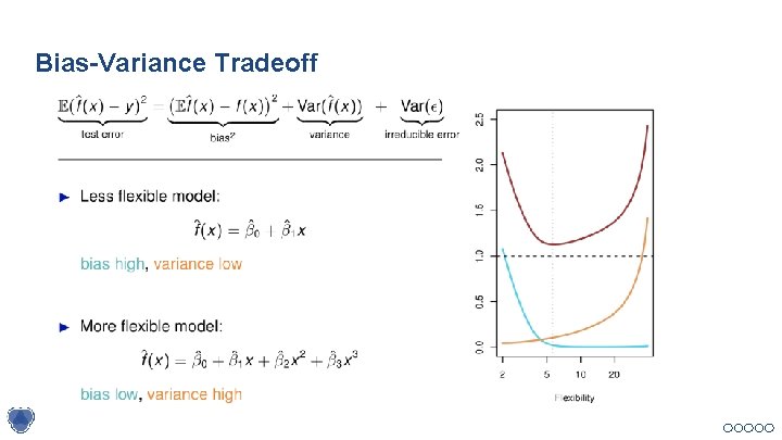
Bias-Variance Tradeoff When evaluating the models we are using, one property that we would often refer to is the biasvariance tradeoff. Bias-variance tradeoff is the property of a set of predictive models where: ● Models with higher flexibility would typically have lower bias and higher variance; ● Models with lower flexibility would typically have higher bias and lower variance. The graph gives a visualization on the outcomes of different bias and variance if we are doing experiment of throwing darts. Graph source: http: //scott. fortmann-roe. com/docs/Bias. Variance. html

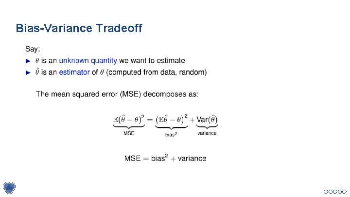
Bias-Variance Tradeoff

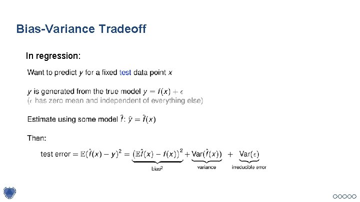
Bias-Variance Tradeoff In regression:

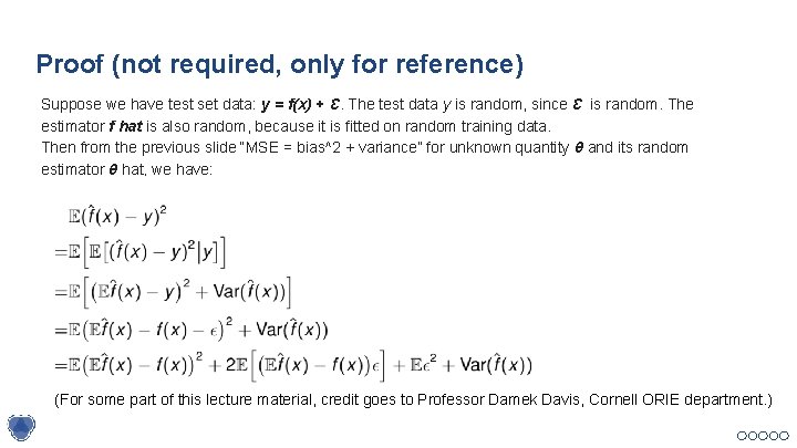
Proof (not required, only for reference) Suppose we have test set data: y = f(x) + Ɛ. The test data y is random, since Ɛ is random. The estimator f hat is also random, because it is fitted on random training data. Then from the previous slide “MSE = bias^2 + variance” for unknown quantity θ and its random estimator θ hat, we have: ε (For some part of this lecture material, credit goes to Professor Damek Davis, Cornell ORIE department. )

Bias-Variance Tradeoff

More Validation Techniques

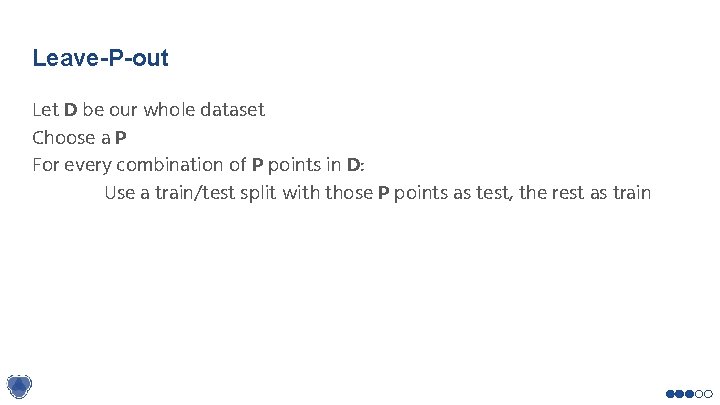
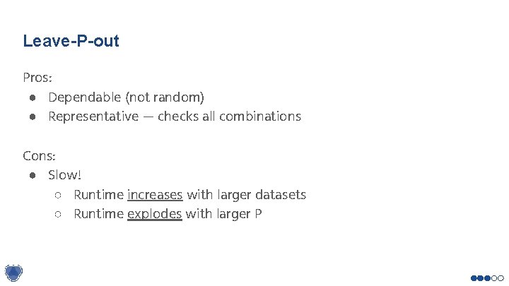
Leave-P-out Let D be our whole dataset Choose a P For every combination of P points in D: Use a train/test split with those P points as test, the rest as train

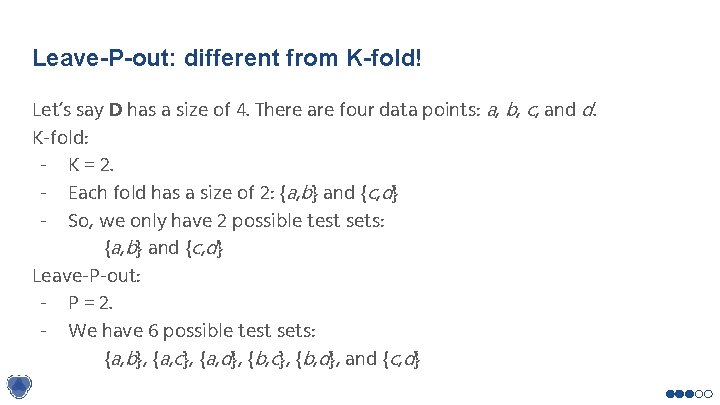
Leave-P-out: different from K-fold! Let’s say D has a size of 4. There are four data points: a, b, c, and d. K-fold: - K = 2. - Each fold has a size of 2: {a, b} and {c, d} - So, we only have 2 possible test sets: {a, b} and {c, d} Leave-P-out: - P = 2. - We have 6 possible test sets: {a, b}, {a, c}, {a, d}, {b, c}, {b, d}, and {c, d}

Leave-P-out Pros: ● Dependable (not random) ● Representative — checks all combinations Cons: ● Slow! ○ Runtime increases with larger datasets ○ Runtime explodes with larger P

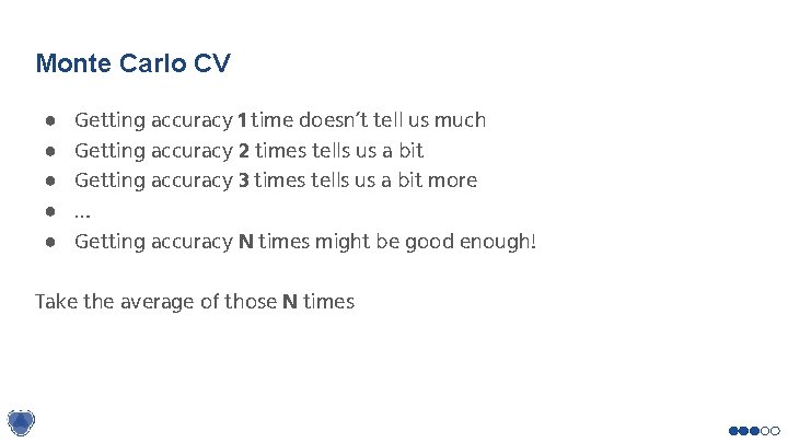
Monte Carlo CV ● ● ● Getting accuracy 1 time doesn’t tell us much Getting accuracy 2 times tells us a bit Getting accuracy 3 times tells us a bit more … Getting accuracy N times might be good enough! Take the average of those N times

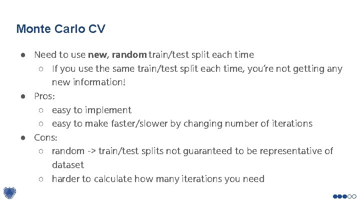
Monte Carlo CV ● Need to use new, random train/test split each time ○ If you use the same train/test split each time, you’re not getting any new information! ● Pros: ○ easy to implement ○ easy to make faster/slower by changing number of iterations ● Cons: ○ random -> train/test splits not guaranteed to be representative of dataset ○ harder to calculate how many iterations you need

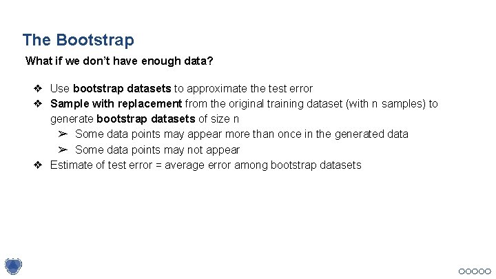
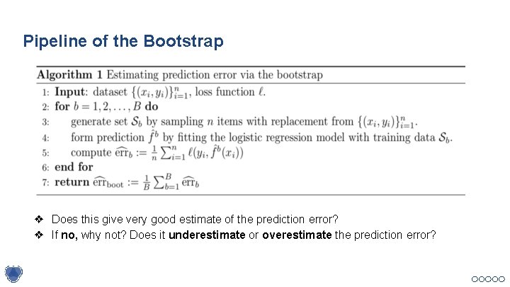
The Bootstrap What if we don’t have enough data? ❖ Use bootstrap datasets to approximate the test error ❖ Sample with replacement from the original training dataset (with n samples) to generate bootstrap datasets of size n ➢ Some data points may appear more than once in the generated data ➢ Some data points may not appear ❖ Estimate of test error = average error among bootstrap datasets

Pipeline of the Bootstrap ❖ Does this give very good estimate of the prediction error? ❖ If no, why not? Does it underestimate or overestimate the prediction error?

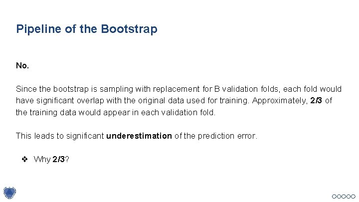
Pipeline of the Bootstrap No. Since the bootstrap is sampling with replacement for B validation folds, each fold would have significant overlap with the original data used for training. Approximately, 2/3 of the training data would appear in each validation fold. This leads to significant underestimation of the prediction error. ❖ Why 2/3?

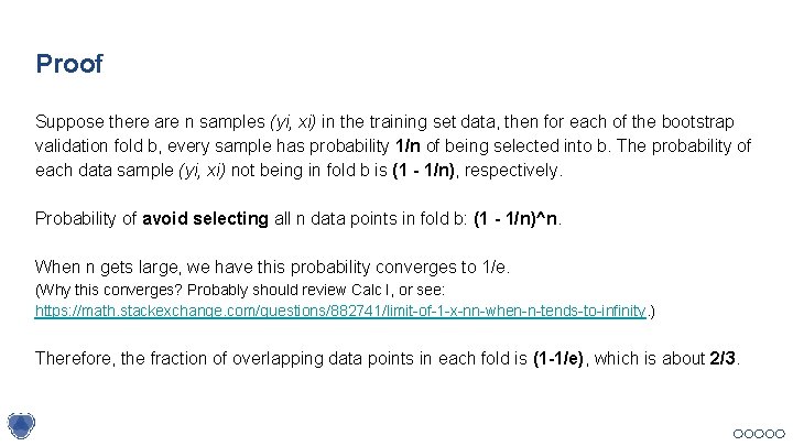
Proof Suppose there are n samples (yi, xi) in the training set data, then for each of the bootstrap validation fold b, every sample has probability 1/n of being selected into b. The probability of each data sample (yi, xi) not being in fold b is (1 - 1/n), respectively. Probability of avoid selecting all n data points in fold b: (1 - 1/n)^n. When n gets large, we have this probability converges to 1/e. (Why this converges? Probably should review Calc I, or see: https: //math. stackexchange. com/questions/882741/limit-of-1 -x-nn-when-n-tends-to-infinity. ) Therefore, the fraction of overlapping data points in each fold is (1 -1/e), which is about 2/3.

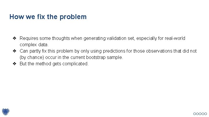
How we fix the problem ❖ Requires some thoughts when generating validation set, especially for real-world complex data. ❖ Can partly fix this problem by only using predictions for those observations that did not (by chance) occur in the current bootstrap sample. ❖ But the method gets complicated.

Bootstrap vs. k-fold In K-fold validation, each of the K folds is distinct from the other (K − 1) folds used for training: there is no overlap. This is crucial for its success in estimating prediction error.

Why we still use bootstrap ❖ Bootstrap allows us to use a computer to mimic the process of obtaining new data sets. ❖ Can be used to quantify the uncertainty associated with a given estimator or statistical learning method. ❖ Provides an estimate of the standard error of a coefficient, or a confidence interval for that coefficient. ➢ i. e. , the variability of the model!

Measures of overfitting ● Compare train accuracy with test accuracy! ● Method 1: Generalization error ○ (Generalization error) = (test error) - (train error) ○ Error introduced from trying to generalize to new data ● Method 2: Prediction variation ○ VAR(predictions for a specific point x) ○ How much do predictions change for point x, based on the training data? Reminder: don’t mix up error and accuracy! They’re nearly equivalent measures, but confusing them in your code can cause problems

Demo

Coming Up • • Assignment 8: Due at 5: 30 pm next Wednesday Next Lecture: Applications of Unsupervised Learning