Lecture 8 Algorithm Efficiency and Simple Sorting Measuring

Lecture 8: Algorithm Efficiency and Simple Sorting

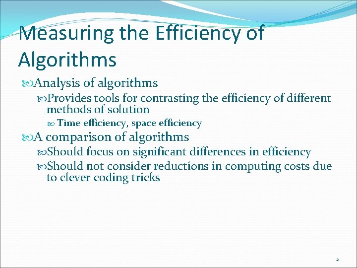
Measuring the Efficiency of Algorithms Analysis of algorithms Provides tools for contrasting the efficiency of different methods of solution Time efficiency, space efficiency A comparison of algorithms Should focus on significant differences in efficiency Should not consider reductions in computing costs due to clever coding tricks 2

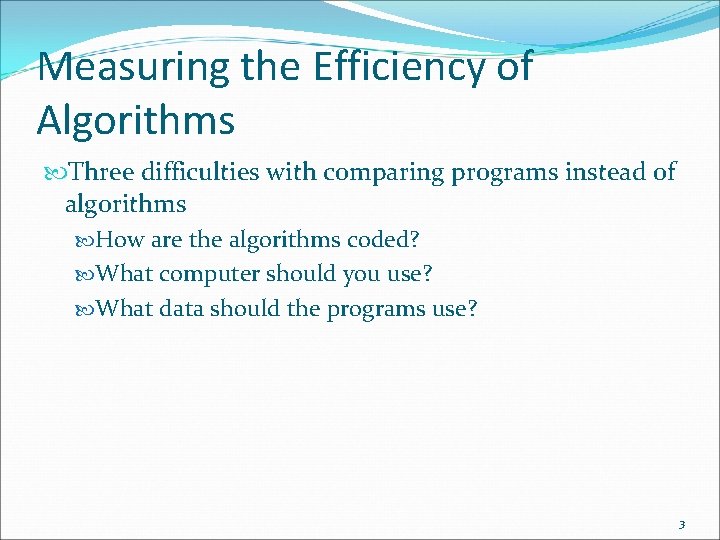
Measuring the Efficiency of Algorithms Three difficulties with comparing programs instead of algorithms How are the algorithms coded? What computer should you use? What data should the programs use? 3

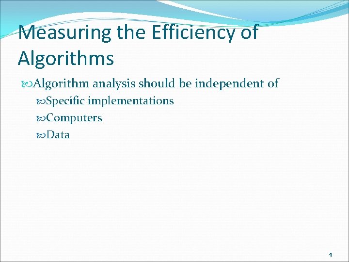
Measuring the Efficiency of Algorithms Algorithm analysis should be independent of Specific implementations Computers Data 4

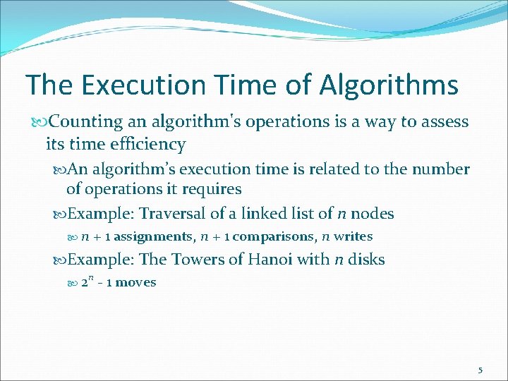
The Execution Time of Algorithms Counting an algorithm's operations is a way to assess its time efficiency An algorithm’s execution time is related to the number of operations it requires Example: Traversal of a linked list of n nodes n + 1 assignments, n + 1 comparisons, n writes Example: The Towers of Hanoi with n disks n 2 - 1 moves 5

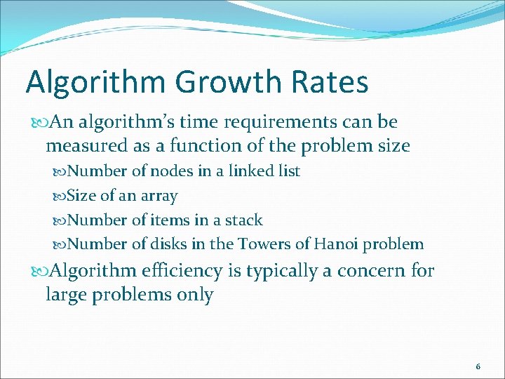
Algorithm Growth Rates An algorithm’s time requirements can be measured as a function of the problem size Number of nodes in a linked list Size of an array Number of items in a stack Number of disks in the Towers of Hanoi problem Algorithm efficiency is typically a concern for large problems only 6

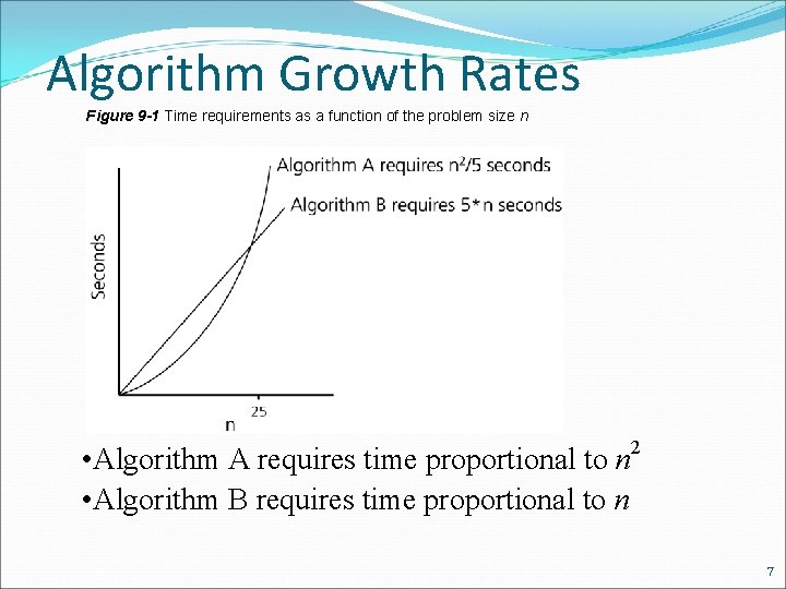
Algorithm Growth Rates Figure 9 -1 Time requirements as a function of the problem size n 2 • Algorithm A requires time proportional to n • Algorithm B requires time proportional to n 7

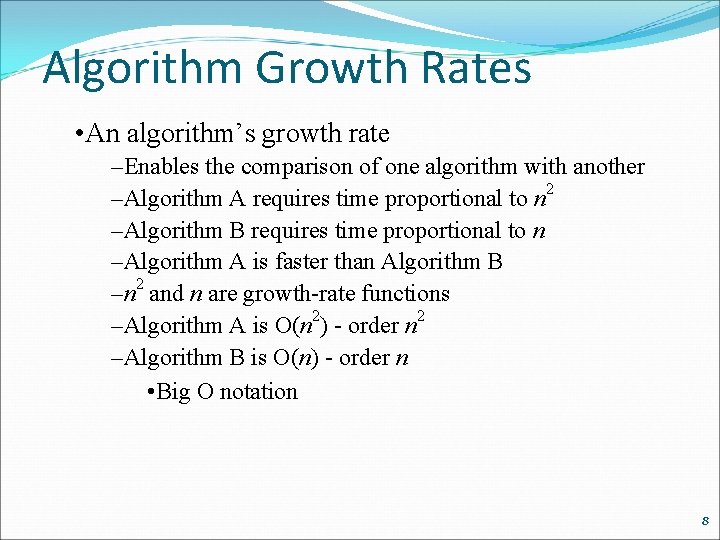
Algorithm Growth Rates • An algorithm’s growth rate –Enables the comparison of one algorithm with another –Algorithm A requires time proportional to n 2 –Algorithm B requires time proportional to n –Algorithm A is faster than Algorithm B –n 2 and n are growth-rate functions –Algorithm A is O(n 2) - order n 2 –Algorithm B is O(n) - order n • Big O notation 8

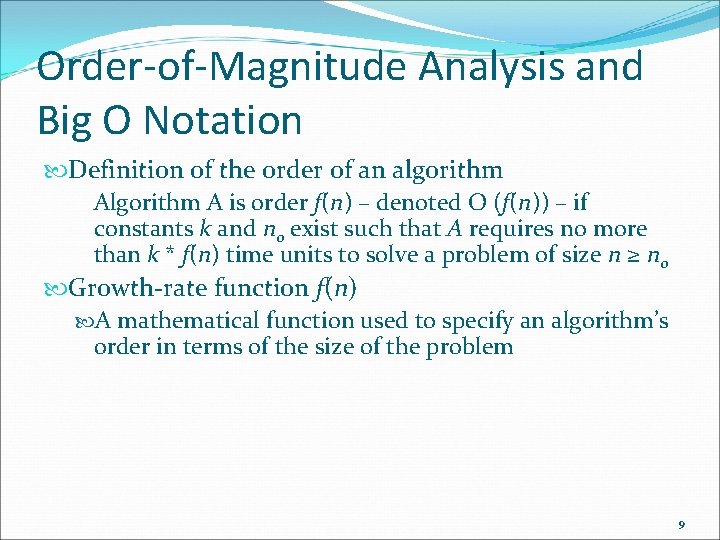
Order-of-Magnitude Analysis and Big O Notation Definition of the order of an algorithm A is order f(n) – denoted O (f(n)) – if constants k and n 0 exist such that A requires no more than k * f(n) time units to solve a problem of size n ≥ n 0 Growth-rate function f(n) A mathematical function used to specify an algorithm’s order in terms of the size of the problem 9

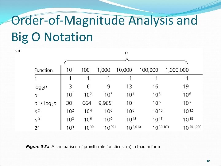
Order-of-Magnitude Analysis and Big O Notation Figure 9 -3 a A comparison of growth-rate functions: (a) in tabular form 10

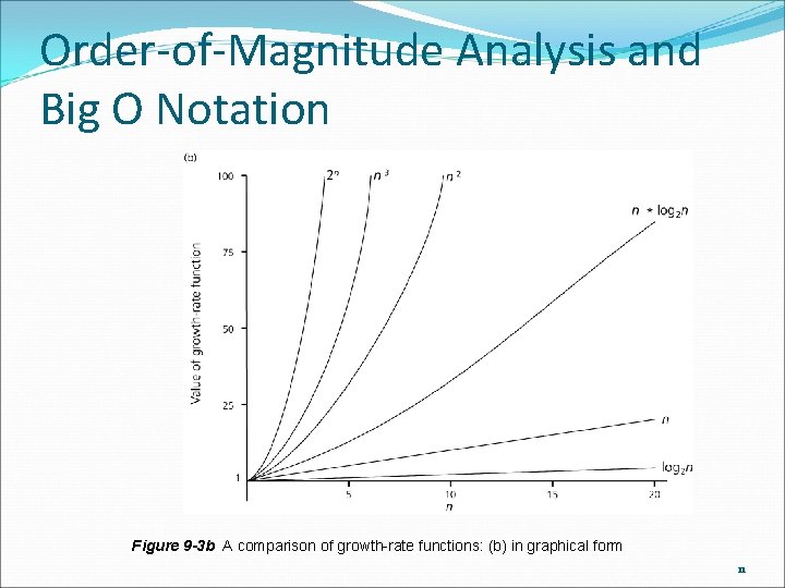
Order-of-Magnitude Analysis and Big O Notation Figure 9 -3 b A comparison of growth-rate functions: (b) in graphical form 11

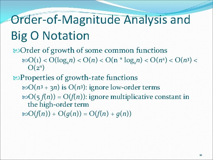
Order-of-Magnitude Analysis and Big O Notation Order of growth of some common functions O(1) < O(log 2 n) < O(n * log 2 n) < O(n 2) < O(n 3) < O(2 n) Properties of growth-rate functions O(n 3 + 3 n) is O(n 3): ignore low-order terms O(5 f(n)) = O(f(n)): ignore multiplicative constant in the high-order term O(f(n)) + O(g(n)) = O(f(n) + g(n)) 12

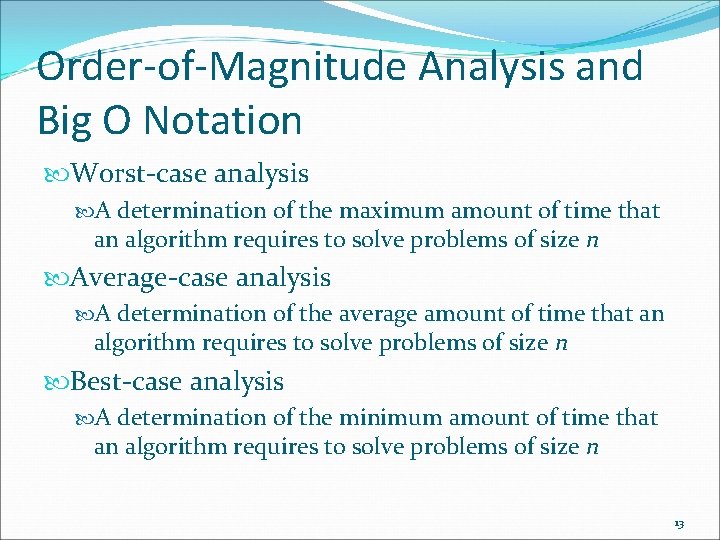
Order-of-Magnitude Analysis and Big O Notation Worst-case analysis A determination of the maximum amount of time that an algorithm requires to solve problems of size n Average-case analysis A determination of the average amount of time that an algorithm requires to solve problems of size n Best-case analysis A determination of the minimum amount of time that an algorithm requires to solve problems of size n 13

Keeping Your Perspective Only significant differences in efficiency are interesting Frequency of operations When choosing an ADT’s implementation, consider how frequently particular ADT operations occur in a given application However, some seldom-used but critical operations must be efficient 14

Keeping Your Perspective If the problem size is always small, you can probably ignore an algorithm’s efficiency Order-of-magnitude analysis focuses on large problems Weigh the trade-offs between an algorithm’s time requirements and its memory requirements Compare algorithms for both style and efficiency 15

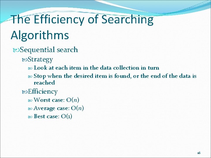
The Efficiency of Searching Algorithms Sequential search Strategy Look at each item in the data collection in turn Stop when the desired item is found, or the end of the data is reached Efficiency Worst case: O(n) Average case: O(n) Best case: O(1) 16

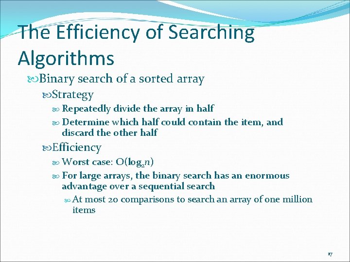
The Efficiency of Searching Algorithms Binary search of a sorted array Strategy Repeatedly divide the array in half Determine which half could contain the item, and discard the other half Efficiency Worst case: O(log 2 n) For large arrays, the binary search has an enormous advantage over a sequential search At most 20 comparisons to search an array of one million items 17

Sorting Algorithms and Their Efficiency Sorting A process that organizes a collection of data into either ascending or descending order The sort key The part of a data item that we consider when sorting a data collection 18

Sorting Algorithms and Their Efficiency Categories of sorting algorithms An internal sort Requires that the collection of data fit entirely in the computer’s main memory An external sort The collection of data will not fit in the computer’s main memory all at once, but must reside in secondary storage 19

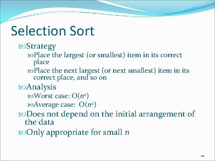
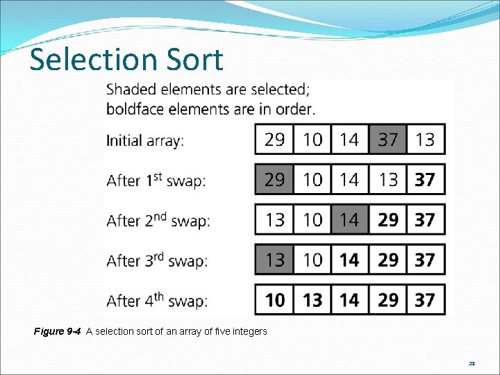
Selection Sort Strategy Place the largest (or smallest) item in its correct place Place the next largest (or next smallest) item in its correct place, and so on Analysis Worst case: O(n 2) Average case: O(n 2) Does not depend on the initial arrangement of the data Only appropriate for small n 20

Selection Sort Figure 9 -4 A selection sort of an array of five integers 21

Algorithm Sorting. cpp void selection(int A[]) { for (int l = array. Size -1; l >= 0; --l) { int LI = l; for (int CI = 0; CI < l; ++CI) { if (A[CI] > A[LI]) LI = CI; } int temp = A[LI]; A[LI]=A[l]; A[l] = temp; } // end for } // end selection. Sort 22

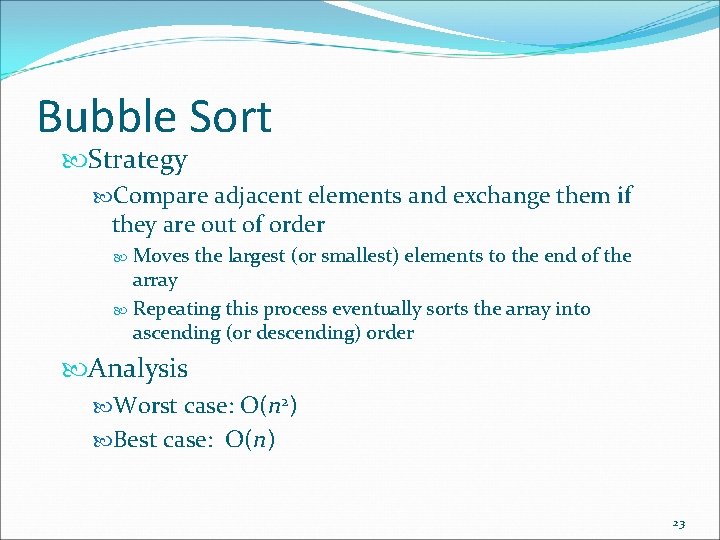
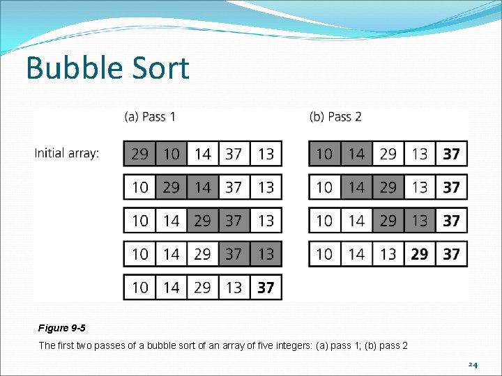
Bubble Sort Strategy Compare adjacent elements and exchange them if they are out of order Moves the largest (or smallest) elements to the end of the array Repeating this process eventually sorts the array into ascending (or descending) order Analysis Worst case: O(n 2) Best case: O(n) 23

Bubble Sort Figure 9 -5 The first two passes of a bubble sort of an array of five integers: (a) pass 1; (b) pass 2 24

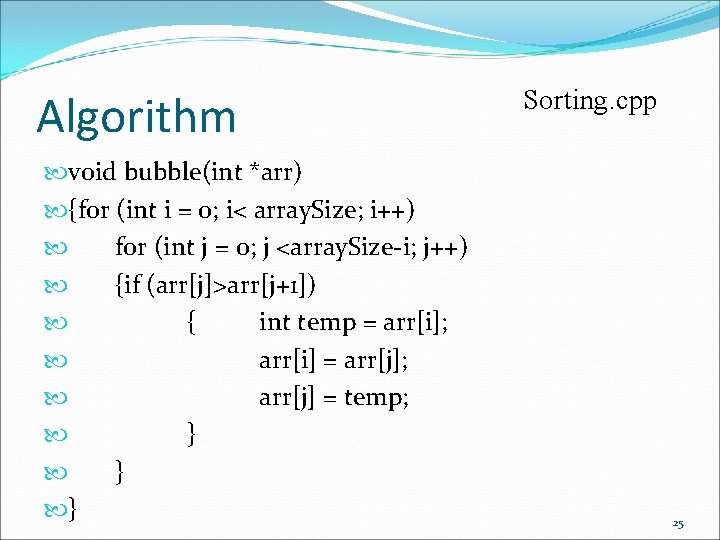
Algorithm void bubble(int *arr) {for (int i = 0; i< array. Size; i++) for (int j = 0; j <array. Size-i; j++) {if (arr[j]>arr[j+1]) { int temp = arr[i]; arr[i] = arr[j]; arr[j] = temp; } } } Sorting. cpp 25

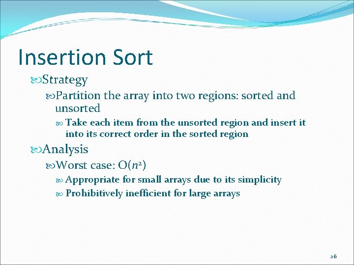
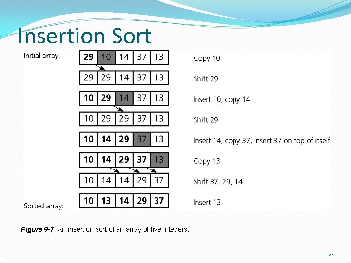
Insertion Sort Strategy Partition the array into two regions: sorted and unsorted Take each item from the unsorted region and insert it into its correct order in the sorted region Analysis Worst case: O(n 2) Appropriate for small arrays due to its simplicity Prohibitively inefficient for large arrays 26

Insertion Sort Figure 9 -7 An insertion sort of an array of five integers. 27

Algorithm Sorting. cpp void insertion(int A[]) { for (int i = 1; i < array. Size; ++i) { int next. Item = A[i]; int loc; for (loc = i; loc > 0; --loc) if (A[loc-1]> next. Item) A[loc] = A[loc-1]; else break; A[loc] = next. Item; } // end for } // end insertion. Sort 28

Mergesort A recursive sorting algorithm Performance is independent of the initial order of the array items Strategy Divide an array into halves Sort each half Merge the sorted halves into one sorted array Divide-and-conquer 29

Mergesort Analysis Worst case: O(n * log 2 n) Average case: O(n * log 2 n) Advantage Mergesort is an extremely fast algorithm Disadvantage Mergesort requires a second array as large as the original array 30

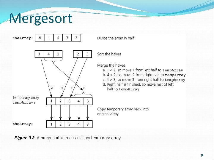
Mergesort Figure 9 -8 A mergesort with an auxiliary temporary array 31

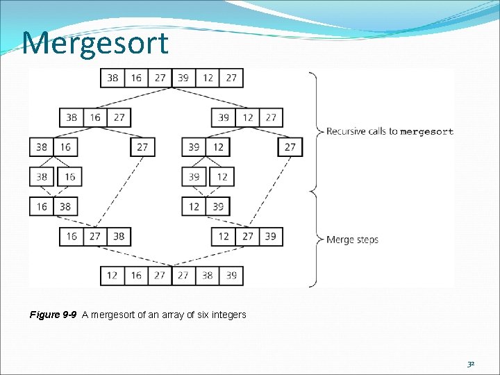
Mergesort Figure 9 -9 A mergesort of an array of six integers 32

The Algorithm void mergesort(int the. Array[], int first, int last) { if (first < last) { int mid = (first + last)/2; // index of midpoint mergesort(the. Array, first, mid); mergesort(the. Array, mid+1, last); merge(the. Array, first, mid, last); } // end if } // end mergesort 33

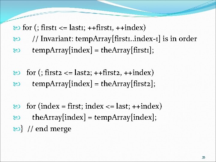
void merge(int the. Array[], int first, int mid, int last) { int temp. Array[array. Size]; // temporary array int first 1 = first; // beginning of first subarray int last 1 = mid; // end of first subarray int first 2 = mid + 1; // beginning of second subarray int last 2 = last; // end of second subarray int index; // next available location in for (index = first 1; (first 1 <= last 1) && (first 2 <= last 2); ++index) { if (the. Array[first 1] < the. Array[first 2]) { temp. Array[index] = the. Array[first 1]; ++first 1; } else { temp. Array[index] = the. Array[first 2]; ++first 2; } // end if } // end for 34

for (; first 1 <= last 1; ++first 1, ++index) // Invariant: temp. Array[first 1. . index-1] is in order temp. Array[index] = the. Array[first 1]; for (; first 2 <= last 2; ++first 2, ++index) temp. Array[index] = the. Array[first 2]; for (index = first; index <= last; ++index) the. Array[index] = temp. Array[index]; } // end merge 35

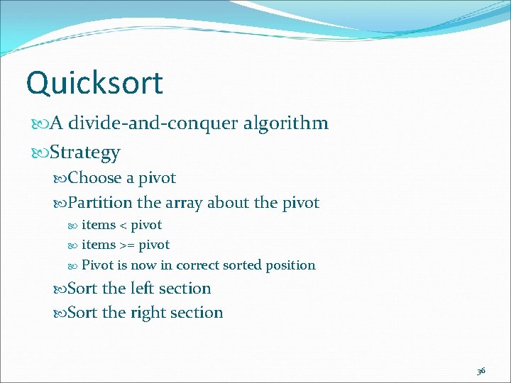
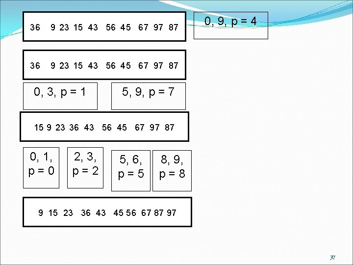
Quicksort A divide-and-conquer algorithm Strategy Choose a pivot Partition the array about the pivot items < pivot items >= pivot Pivot is now in correct sorted position Sort the left section Sort the right section 36

36 9 23 15 43 56 45 67 97 87 0, 3, p = 1 0, 9, p = 4 5, 9, p = 7 15 9 23 36 43 56 45 67 97 87 0, 1, p=0 2, 3, p=2 5, 6, p=5 8, 9, p=8 9 15 23 36 43 45 56 67 87 97 37

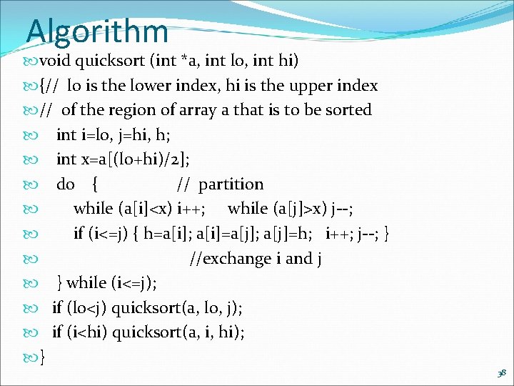
Algorithm void quicksort (int *a, int lo, int hi) {// lo is the lower index, hi is the upper index // of the region of array a that is to be sorted int i=lo, j=hi, h; int x=a[(lo+hi)/2]; do { // partition while (a[i]<x) i++; while (a[j]>x) j--; if (i<=j) { h=a[i]; a[i]=a[j]; a[j]=h; i++; j--; } //exchange i and j } while (i<=j); if (lo<j) quicksort(a, lo, j); if (i<hi) quicksort(a, i, hi); } 38

Quicksort Analysis Average case: O(n * log 2 n) Worst case: O(n 2) When the array is already sorted and the smallest item is chosen as the pivot Quicksort is usually extremely fast in practice Even if the worst case occurs, quicksort’s performance is acceptable for moderately large arrays 39

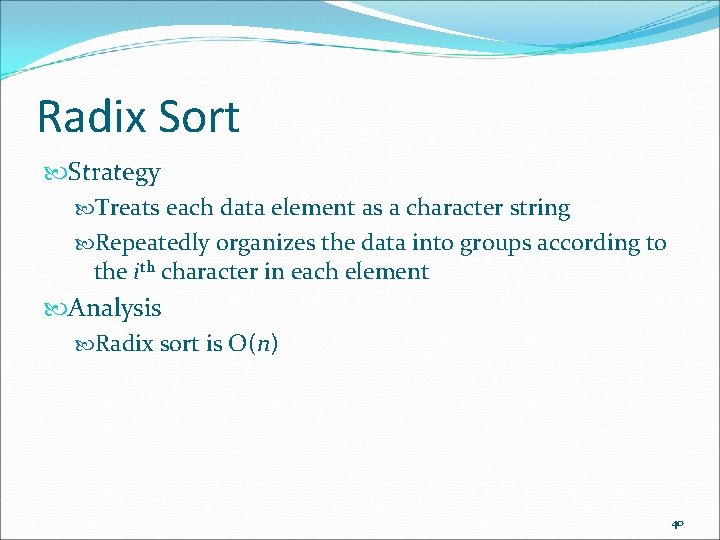
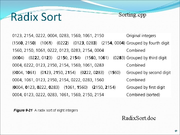
Radix Sort Strategy Treats each data element as a character string Repeatedly organizes the data into groups according to the ith character in each element Analysis Radix sort is O(n) 40

Radix Sorting. cpp Figure 9 -21 A radix sort of eight integers Radix. Sort. doc 41

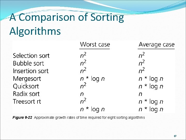
A Comparison of Sorting Algorithms Figure 9 -22 Approximate growth rates of time required for eight sorting algorithms 42

The STL Sorting Algorithms Some sort functions in the STL library header <algorithm> sort Sorts a range of elements in ascending order by default stable_sort Sorts as above, but preserves original ordering of equivalent elements 43

The STL Sorting Algorithms partial_sort Sorts a range of elements and places them at the beginning of the range nth_element Partitions the elements of a range about the nth element The two subranges are not sorted partition Partitions the elements of a range according to a given predicate 44

Summary Order-of-magnitude analysis and Big O notation measure an algorithm’s time requirement as a function of the problem size by using a growthrate function To compare the efficiency of algorithms Examine growth-rate functions when problems are large Consider only significant differences in growth-rate functions 45

Summary Worst-case and average-case analyses Worst-case analysis considers the maximum amount of work an algorithm will require on a problem of a given size Average-case analysis considers the expected amount of work that an algorithm will require on a problem of a given size 46

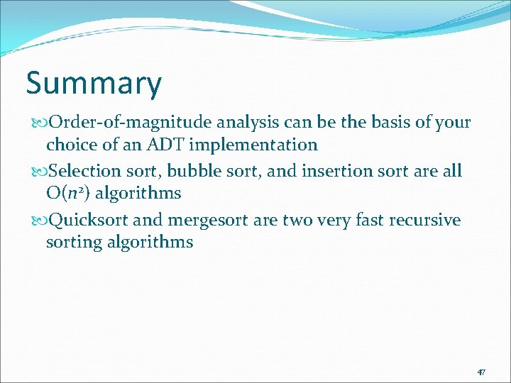
Summary Order-of-magnitude analysis can be the basis of your choice of an ADT implementation Selection sort, bubble sort, and insertion sort are all O(n 2) algorithms Quicksort and mergesort are two very fast recursive sorting algorithms 47