Lecture 8 1 Parallel Algorithms focus on sorting

Lecture 8 -1 : Parallel Algorithms (focus on sorting algorithms) Courtesy : Prof. Chowdhury(SUNY-SB) and Prof. Grossman(UW)’s course note slides are used in this lecture note

Parallel/Distributed Algorithms n Parallel program(algorithm) n n n A program (algorithm) is divided into multiple processes(threads) which are run on multiple processors The processors normally are in one machine execute one program at a time have high speed communications between them Distributed program(algorithm) n n A program (algorithm) is divided into multiple processes which are run on multiple distinct machines The multiple machines are usual connected by network. Machines used typically are workstations running multiple programs.

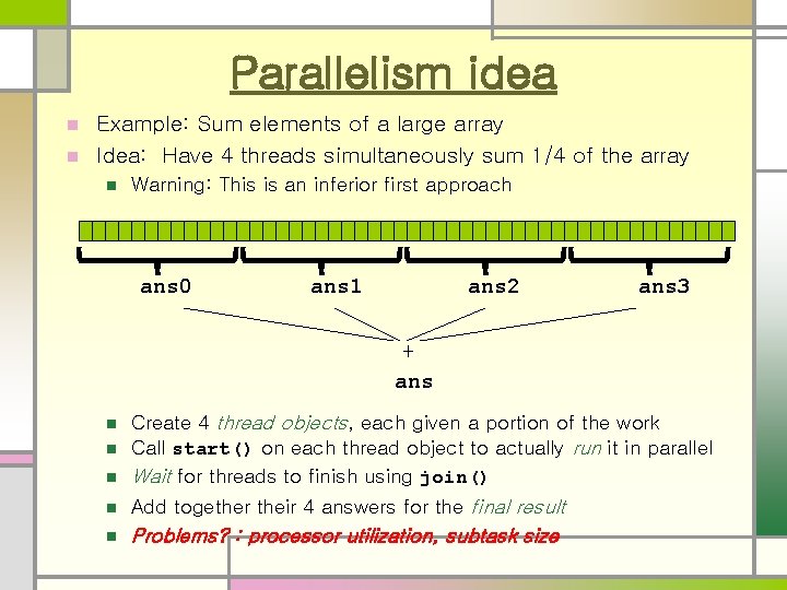
Parallelism idea Example: Sum elements of a large array n Idea: Have 4 threads simultaneously sum 1/4 of the array n n Warning: This is an inferior first approach ans 0 ans 1 ans 2 ans 3 + ans n Create 4 thread objects, each given a portion of the work Call start() on each thread object to actually run it in parallel Wait for threads to finish using join() n Add together their 4 answers for the final result n Problems? : processor utilization, subtask size n n

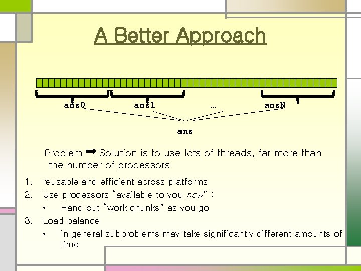
A Better Approach ans 0 ans 1 … ans. N ans Problem Solution is to use lots of threads, far more than the number of processors 1. 2. 3. reusable and efficient across platforms Use processors “available to you now” : • Hand out “work chunks” as you go Load balance • in general subproblems may take significantly different amounts of time

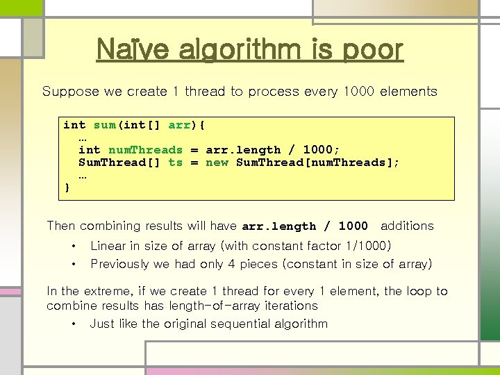
Naïve algorithm is poor Suppose we create 1 thread to process every 1000 elements int sum(int[] arr){ … int num. Threads = arr. length / 1000; Sum. Thread[] ts = new Sum. Thread[num. Threads]; … } Then combining results will have arr. length / 1000 additions • • Linear in size of array (with constant factor 1/1000) Previously we had only 4 pieces (constant in size of array) In the extreme, if we create 1 thread for every 1 element, the loop to combine results has length-of-array iterations • Just like the original sequential algorithm

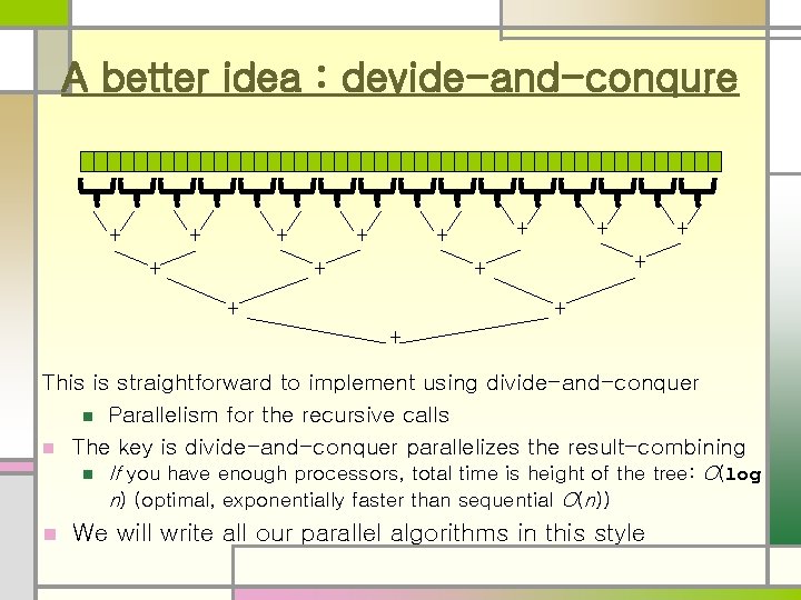
A better idea : devide-and-conqure + + + + This is straightforward to implement using divide-and-conquer n Parallelism for the recursive calls n The key is divide-and-conquer parallelizes the result-combining n If you have enough processors, total time is height of the tree: O(log n) (optimal, exponentially faster than sequential O(n)) n We will write all our parallel algorithms in this style

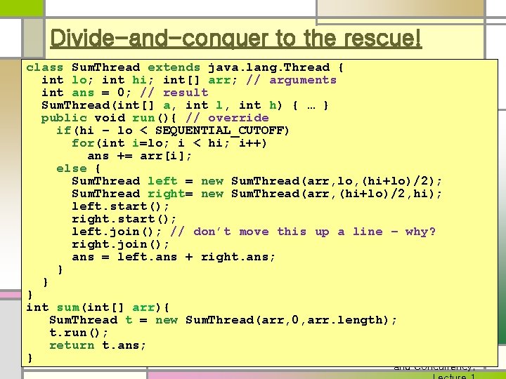
Divide-and-conquer to the rescue! class Sum. Thread extends java. lang. Thread { int lo; int hi; int[] arr; // arguments int ans = 0; // result Sum. Thread(int[] a, int l, int h) { … } public void run(){ // override if(hi – lo < SEQUENTIAL_CUTOFF) for(int i=lo; i < hi; i++) ans += arr[i]; n And using recursive divide-and-conquer else { Sum. Thread left natural = new Sum. Thread(arr, lo, (hi+lo)/2); makes this Sum. Thread right= new Sum. Thread(arr, (hi+lo)/2, hi); nleft. start(); Easier to write and more efficient right. start(); asymptotically! left. join(); // don’t move this up a line – why? right. join(); ans = left. ans + right. ans; } } } int sum(int[] arr){ Sum. Thread t = new Sum. Thread(arr, 0, arr. length); t. run(); return t. ans; 7 Sophomoric Parallelism } The key is to do the result-combining in parallel as well and Concurrency,

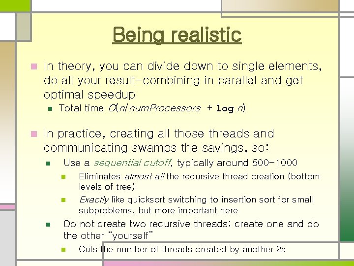
Being realistic n In theory, you can divide down to single elements, do all your result-combining in parallel and get optimal speedup n n Total time O(n/num. Processors + log n) In practice, creating all those threads and communicating swamps the savings, so: n Use a sequential cutoff, typically around 500 -1000 n Eliminates almost all the recursive thread creation (bottom n n levels of tree) Exactly like quicksort switching to insertion sort for small subproblems, but more important here Do not create two recursive threads; create one and do the other “yourself” n Cuts the number of threads created by another 2 x

Similar Problems n Maximum or minimum element n Is there an element satisfying some property n n (e. g. , is there a 17)? Left-most element satisfying some property n (e. g. , first 17) n Corners of a rectangle containing all points (a bounding box) n Counts, for example, number of strings that start with a vowel Computations of this form are called reductions

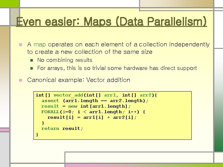
Even easier: Maps (Data Parallelism) n A map operates on each element of a collection independently to create a new collection of the same size n n n No combining results For arrays, this is so trivial some hardware has direct support Canonical example: Vector addition int[] vector_add(int[] arr 1, int[] arr 2){ assert (arr 1. length == arr 2. length); result = new int[arr 1. length]; FORALL(i=0; i < arr 1. length; i++) { result[i] = arr 1[i] + arr 2[i]; } return result; }

Maps and reductions: the “workhorses” of parallel programming n By far the two most important and common patterns n Two more-advanced patterns in next lecture n Learn to recognize when an algorithm can be written in terms of maps and reductions n Use maps and reductions to describe (parallel) algorithms

Divide-and-Conquer in more detail

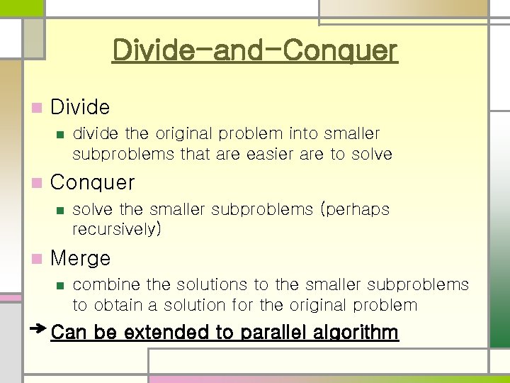
Divide-and-Conquer n Divide n n Conquer n n divide the original problem into smaller subproblems that are easier are to solve the smaller subproblems (perhaps recursively) Merge n combine the solutions to the smaller subproblems to obtain a solution for the original problem Can be extended to parallel algorithm

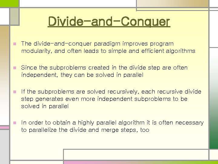
Divide-and-Conquer n The divide-and-conquer paradigm improves program modularity, and often leads to simple and efficient algorithms n Since the subproblems created in the divide step are often independent, they can be solved in parallel n If the subproblems are solved recursively, each recursive divide step generates even more independent subproblems to be solved in parallel n In order to obtain a highly parallel algorithm it is often necessary to parallelize the divide and merge steps, too

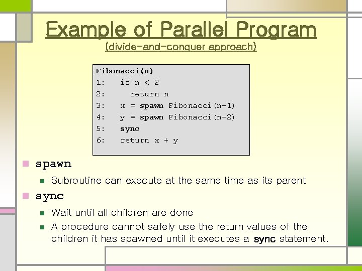
Example of Parallel Program (divide-and-conquer approach) Fibonacci(n) 1: if n < 2 2: return n 3: x = spawn Fibonacci(n-1) 4: y = spawn Fibonacci(n-2) 5: sync 6: return x + y n spawn n n Subroutine can execute at the same time as its parent sync n n Wait until all children are done A procedure cannot safely use the return values of the children it has spawned until it executes a sync statement.

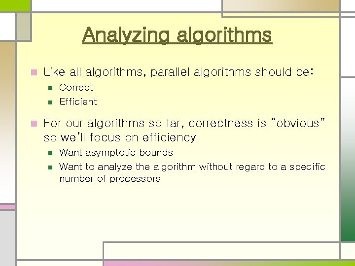
Analyzing algorithms n Like all algorithms, parallel algorithms should be: n n n Correct Efficient For our algorithms so far, correctness is “obvious” so we’ll focus on efficiency n n Want asymptotic bounds Want to analyze the algorithm without regard to a specific number of processors

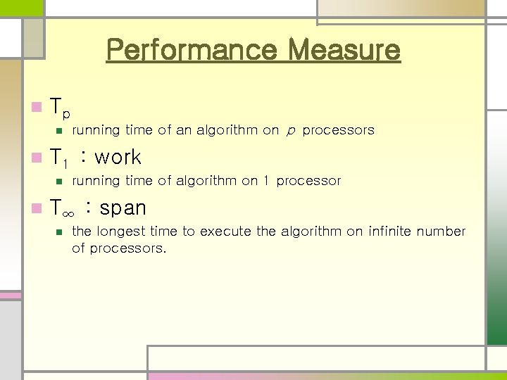
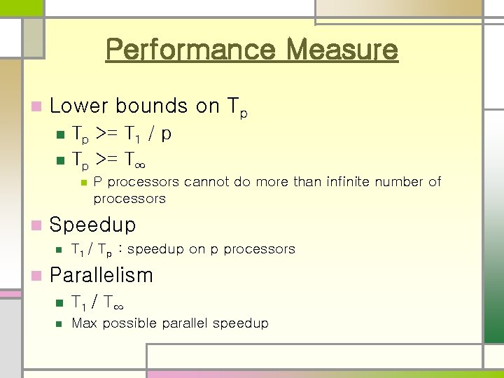
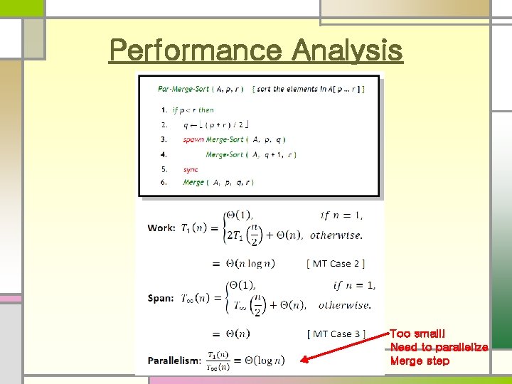
Performance Measure n Tp n n T 1 : work n n running time of an algorithm on p processors running time of algorithm on 1 processor T∞ : span n the longest time to execute the algorithm on infinite number of processors.

Performance Measure n Lower bounds on Tp n n Tp >= T 1 / p Tp >= T∞ n n Speedup n n P processors cannot do more than infinite number of processors T 1 / Tp : speedup on p processors Parallelism n T 1 / T ∞ n Max possible parallel speedup

Related Sorting Algorithms n n Sort an array A[1, …, n] of n keys (using p<=n processors) Examples of divide-and-conquer methods n n Merge-sort Quick-sort

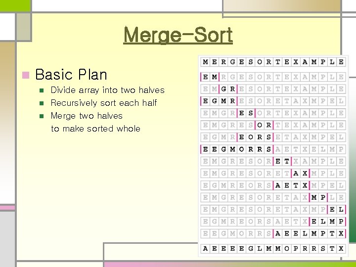
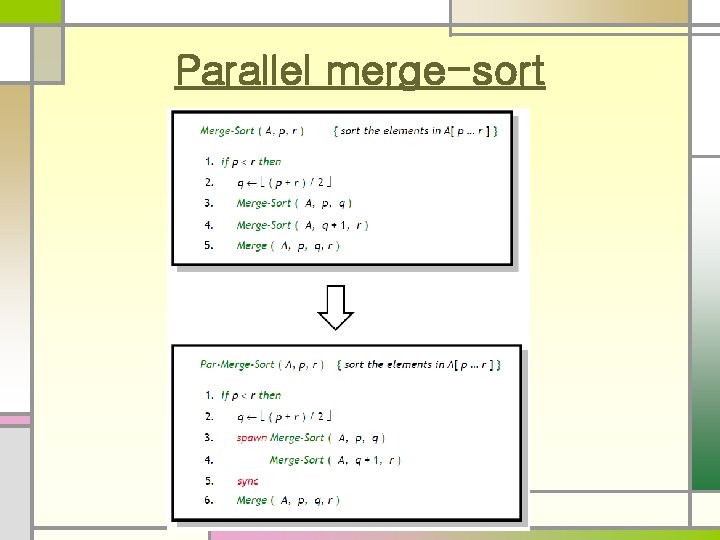
Merge-Sort n Basic Plan n Divide array into two halves Recursively sort each half Merge two halves to make sorted whole

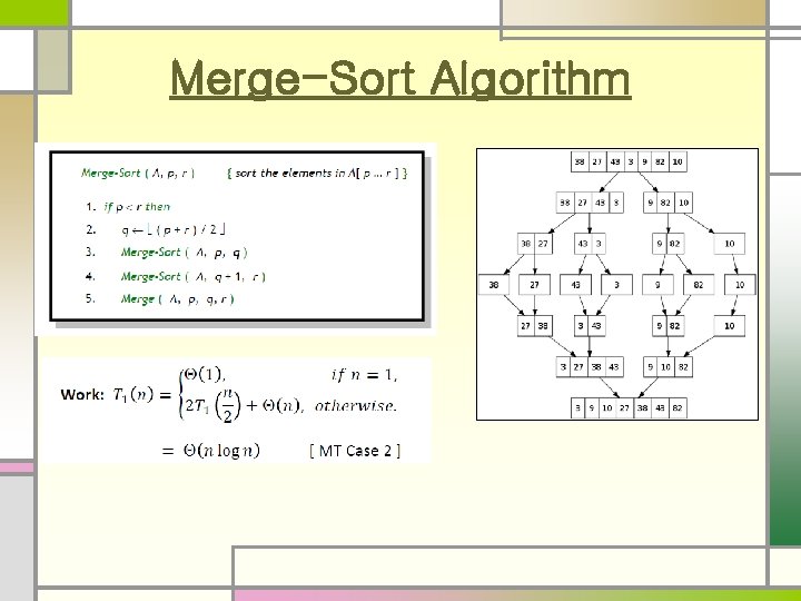
Merge-Sort Algorithm

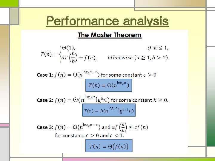
Performance analysis

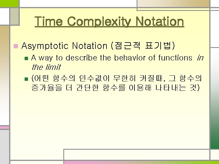
Time Complexity Notation n Asymptotic Notation (점근적 표기법) n A way to describe the behavior of functions in the limit n (어떤 함수의 인수값이 무한히 커질때, 그 함수의 증가율을 더 간단한 함수를 이용해 나타내는 것)

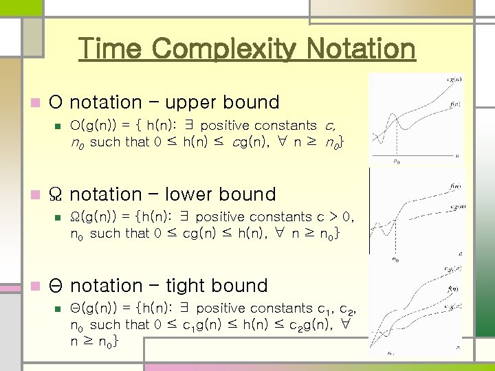
Time Complexity Notation n O notation – upper bound n n Ω notation – lower bound n n O(g(n)) = { h(n): ∃ positive constants c, n 0 such that 0 ≤ h(n) ≤ cg(n), ∀ n ≥ n 0} Ω(g(n)) = {h(n): ∃ positive constants c > 0, n 0 such that 0 ≤ cg(n) ≤ h(n), ∀ n ≥ n 0} Θ notation – tight bound n Θ(g(n)) = {h(n): ∃ positive constants c 1, c 2, n 0 such that 0 ≤ c 1 g(n) ≤ h(n) ≤ c 2 g(n), ∀ n ≥ n 0 }

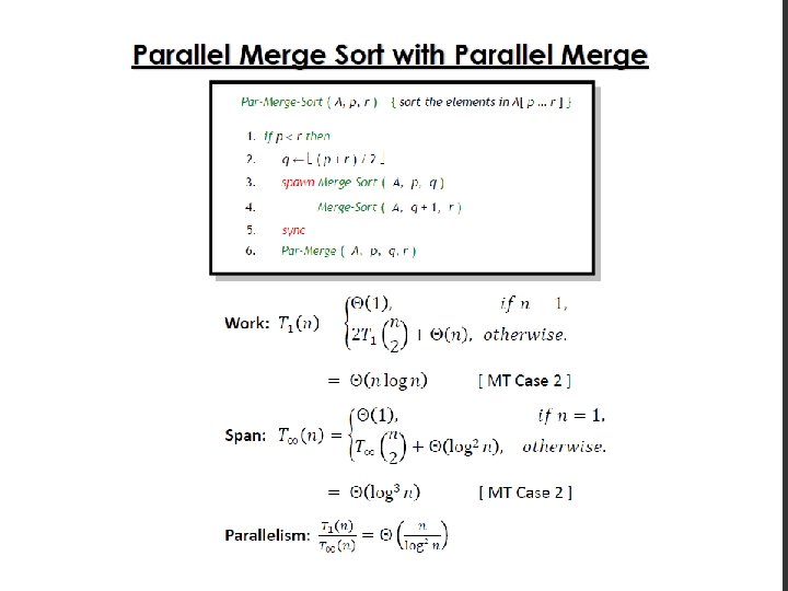
Parallel merge-sort

Performance Analysis Too small! Need to parallelize Merge step

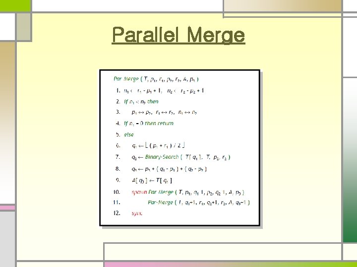
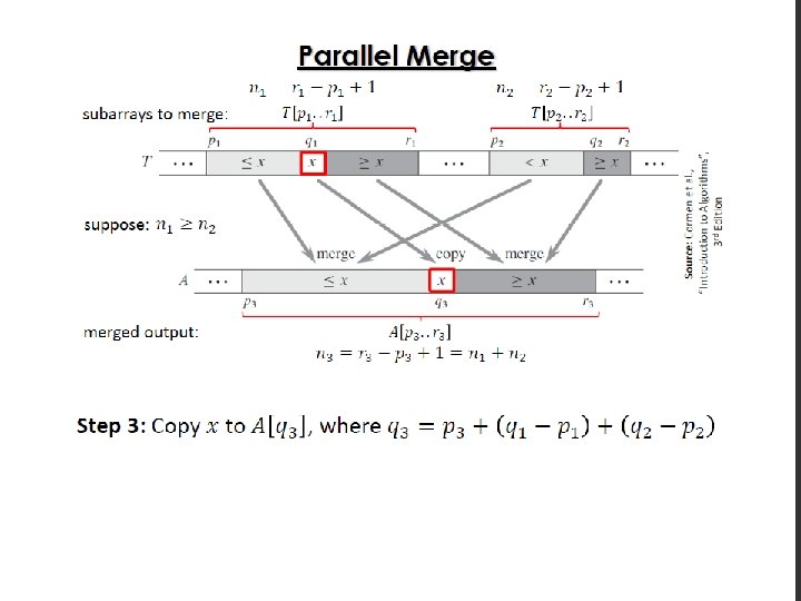
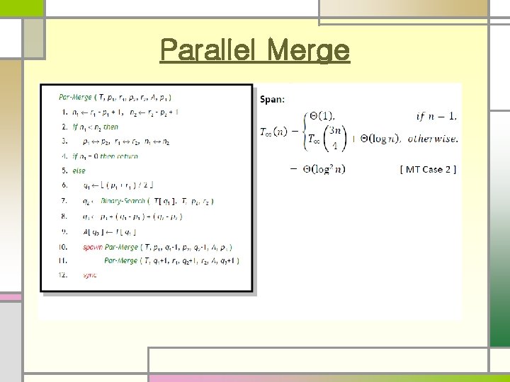
Parallel Merge

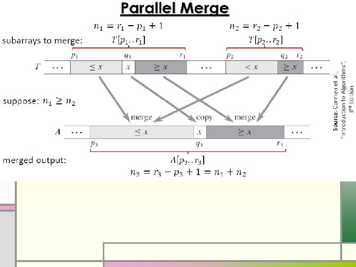
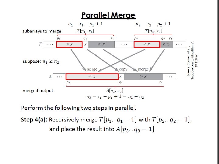
Parallel merge

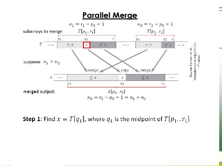
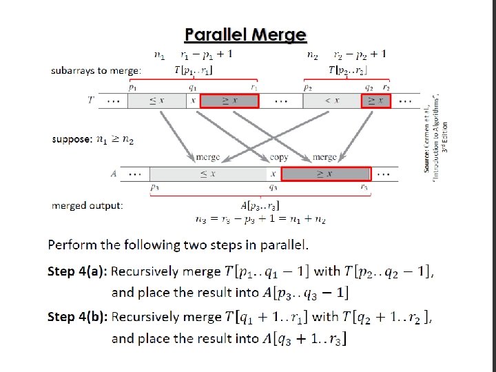
Parallel Merge

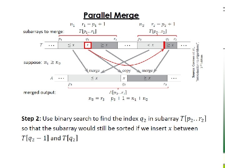
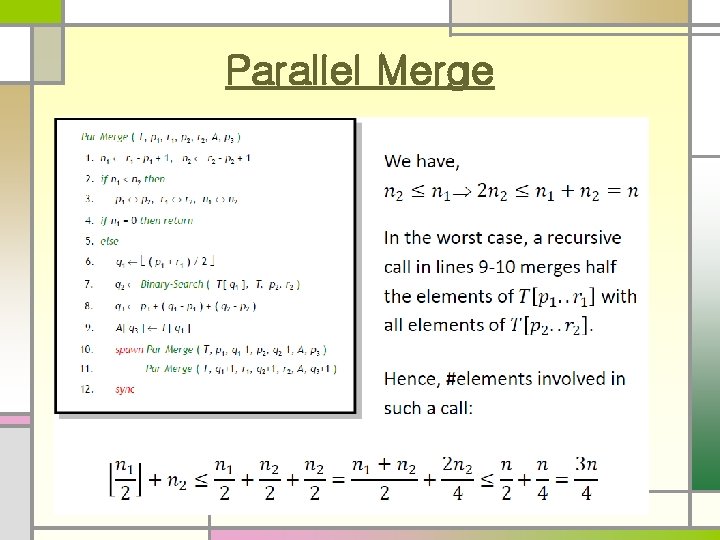
Parallel Merge

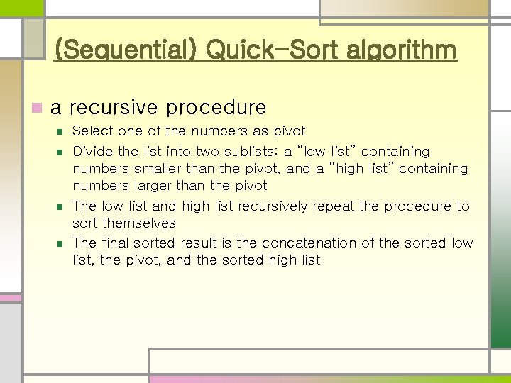
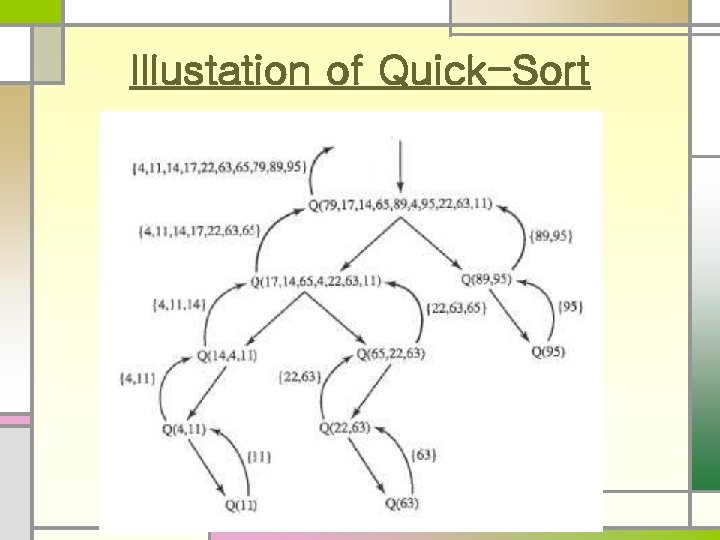
(Sequential) Quick-Sort algorithm n a recursive procedure n n Select one of the numbers as pivot Divide the list into two sublists: a “low list” containing numbers smaller than the pivot, and a “high list” containing numbers larger than the pivot The low list and high list recursively repeat the procedure to sort themselves The final sorted result is the concatenation of the sorted low list, the pivot, and the sorted high list

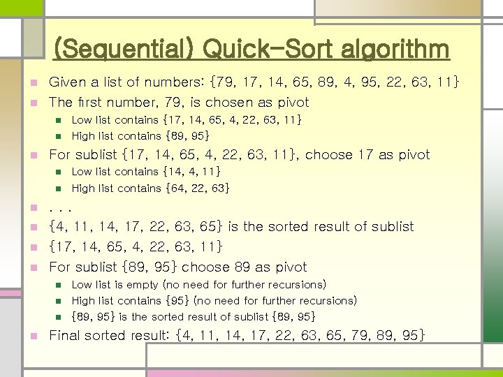
(Sequential) Quick-Sort algorithm Given a list of numbers: {79, 17, 14, 65, 89, 4, 95, 22, 63, 11} n The first number, 79, is chosen as pivot n n Low list contains {17, 14, 65, 4, 22, 63, 11} High list contains {89, 95} For sublist {17, 14, 65, 4, 22, 63, 11}, choose 17 as pivot n n Low list contains {14, 4, 11} High list contains {64, 22, 63} . . . n {4, 11, 14, 17, 22, 63, 65} is the sorted result of sublist n {17, 14, 65, 4, 22, 63, 11} n For sublist {89, 95} choose 89 as pivot n n n Low list is empty (no need for further recursions) High list contains {95} (no need for further recursions) {89, 95} is the sorted result of sublist {89, 95} Final sorted result: {4, 11, 14, 17, 22, 63, 65, 79, 89, 95}

Illustation of Quick-Sort

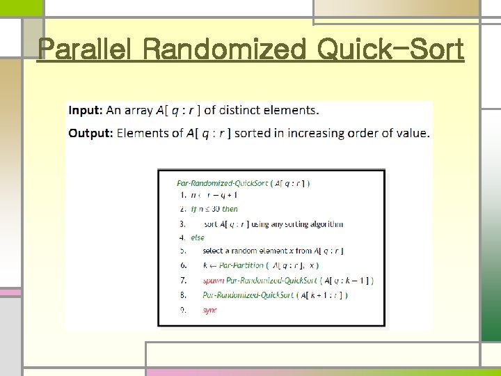
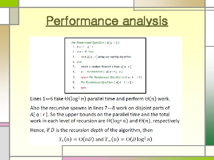
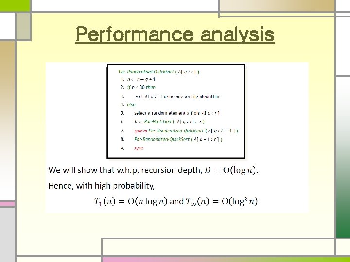
Randomized quick-sort Par-Randomized-Quick. Sort ( A[ q : r ] ) 1. n <- r ― q + 1 2. if n <= 30 then 3. sort A[ q : r ] using any sorting algorithm 4. else 5. select a random element x from A[ q : r ] 6. k <- Par-Partition ( A[ q : r ], x ) 7. spawn Par-Randomized-Quick. Sort ( A[ q : k ― 1 ] ) 8. Par-Randomized-Quick. Sort ( A[ k + 1 : r ] ) 9. sync • Worst-Case Time Complexity of Quick-Sort : O(N^2) • Average Time Complexity of Sequential Randomized Quick-Sort : O(Nlog. N) (recursion depth of line 7 -8 is roughly O(log. N). Line 5 takes O(N))

Parallel Randomized Quick-Sort

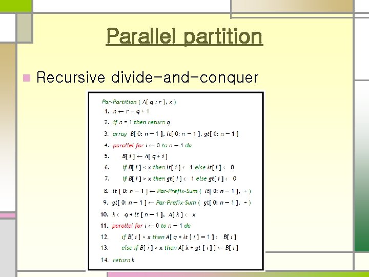
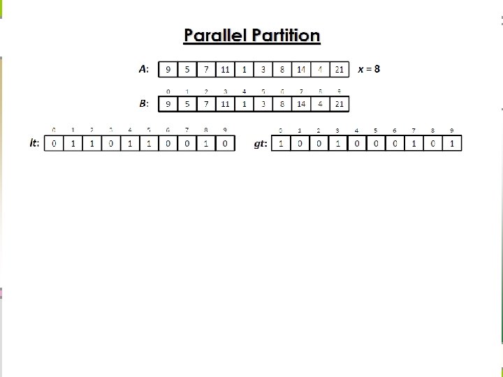
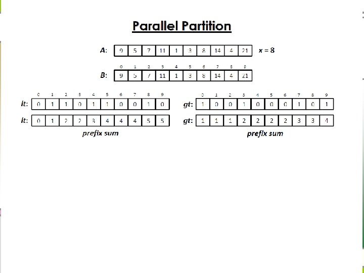
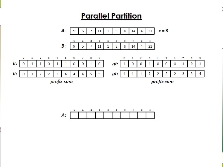
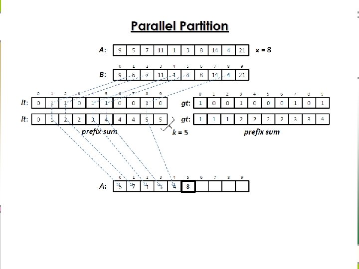
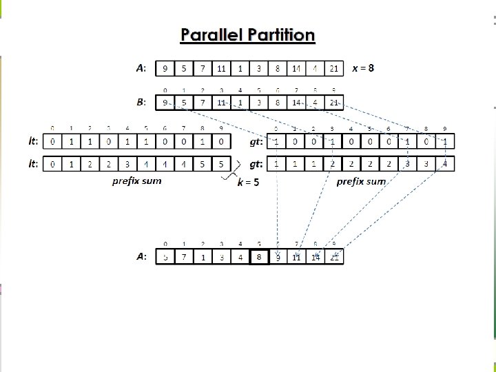
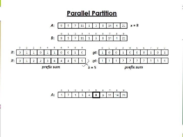
Parallel partition n Recursive divide-and-conquer

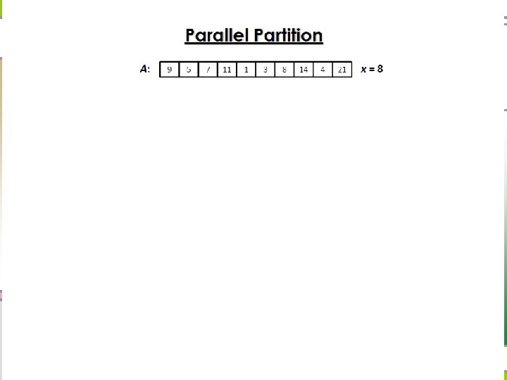
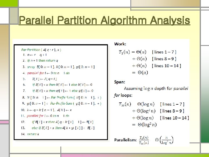
Parallel Partition Algorithm Analysis

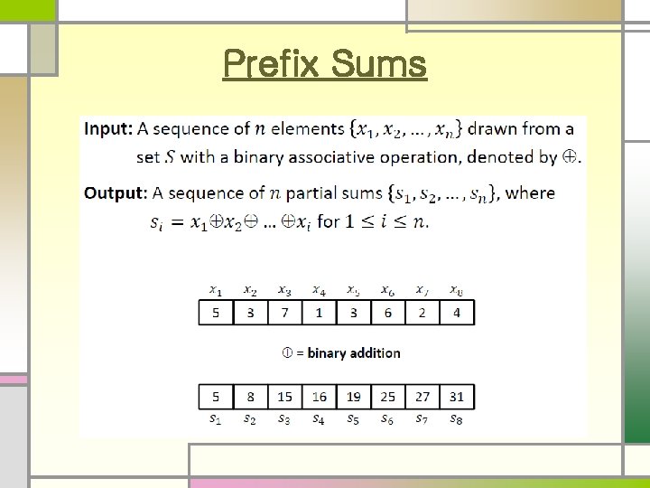
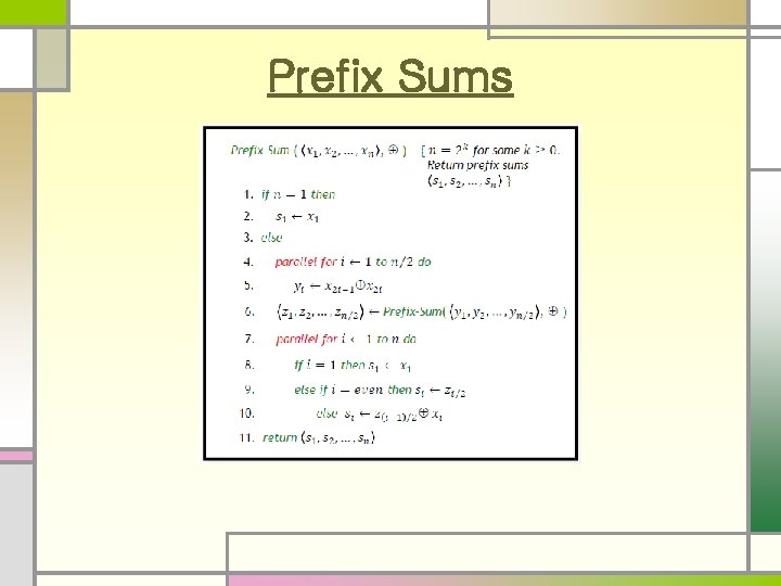
Prefix Sums

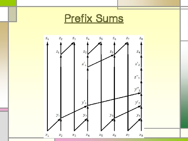
Prefix Sums

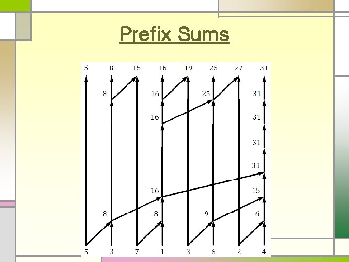
Prefix Sums

Prefix Sums

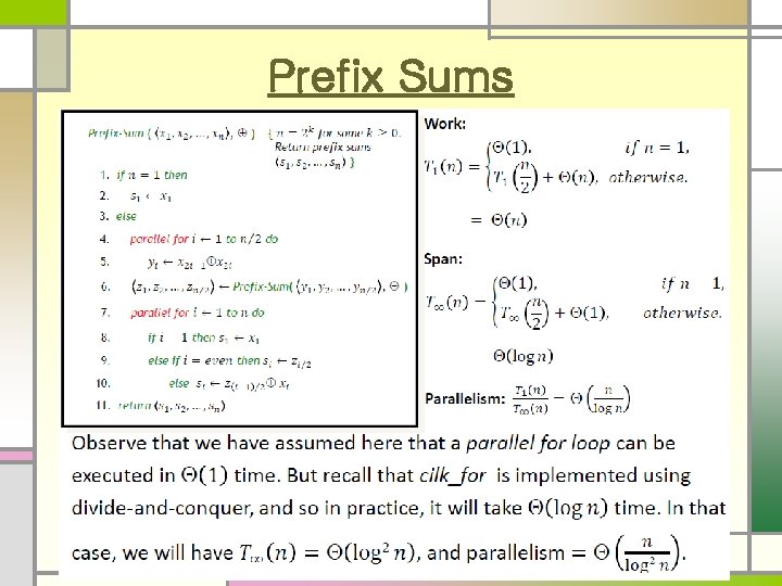
Prefix Sums

Performance analysis

Performance analysis