Lecture 7Image Relaxation Restoration and Feature Extraction ch

Lecture 7—Image Relaxation: Restoration and Feature Extraction ch. 6 of Machine Vision by Wesley E. Snyder & Hairong Qi Spring 2016 18 -791 (CMU ECE) : 42 -735 (CMU BME) : Bio. E 2630 (Pitt) Dr. John Galeotti The content of these slides by John Galeotti, © 2012 - 2016 Carnegie Mellon University (CMU), was made possible in part by NIH NLM contract# HHSN 276201000580 P, and is licensed under a Creative Commons Attribution-Non. Commercial 3. 0 Unported License. To view a copy of this license, visit http: //creativecommons. org/licenses/by-nc/3. 0/ or send a letter to Creative Commons, 171 2 nd Street, Suite 300, San Francisco, California, 94105, USA. Permissions beyond the scope of this license may be available either from CMU or by emailing itk@galeotti. net. The most recent version of these slides may be accessed online via http: //itk. galeotti. net/

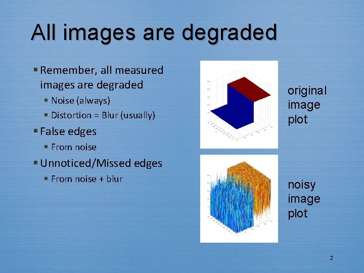
All images are degraded § Remember, all measured images are degraded § Noise (always) § Distortion = Blur (usually) § False edges original image plot § From noise § Unnoticed/Missed edges § From noise + blur noisy image plot 2

We need an “un-degrader”… §To extract “clean” features for segmentation, registration, etc. §Restoration § A-posteriori image restoration § Removes degradations from images §Feature extraction § Iterative image feature extraction § Extracts features from noisy images 3

Image relaxation § The basic operation performed by: § Restoration § Feature extraction (of the type in ch. 6) § An image relaxation process is a multistep algorithm with the properties that: § The output of a step is the same form as the input (e. g. , 2562 image to 2562 image) § Allows iteration § It converges to a bounded result § The operation on any pixel is dependent only on those pixels in some well defined, finite neighborhood of that pixel. (optional) 4

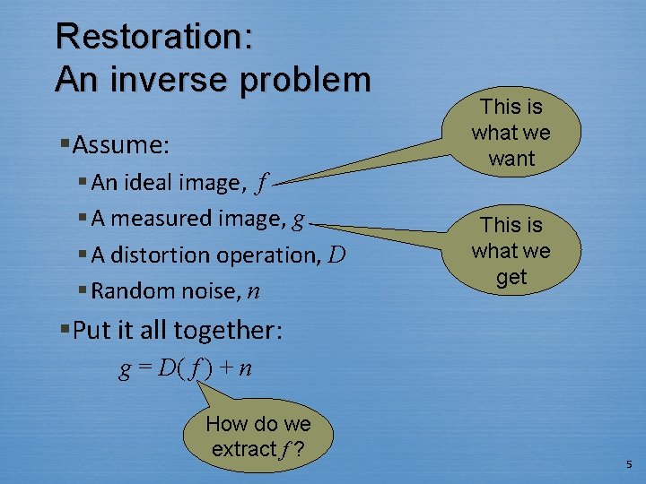
Restoration: An inverse problem §Assume: § An ideal image, f § A measured image, g § A distortion operation, D § Random noise, n This is what we want This is what we get §Put it all together: g = D( f ) + n How do we extract f ? 5

Restoration is ill-posed §Even without noise §Even if the distortion is linear blur § Inverting linear blur = deconvolution §But we want restoration to be well-posed… 6

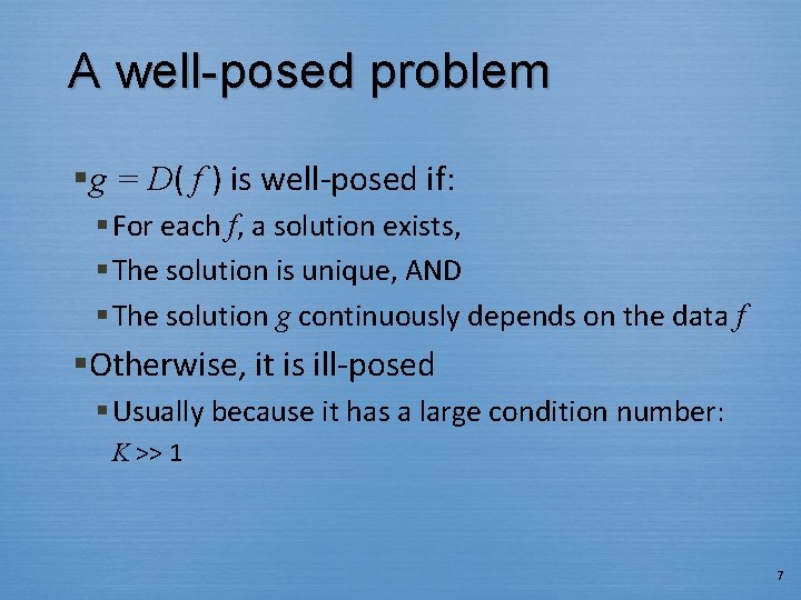
A well-posed problem §g = D( f ) is well-posed if: § For each f, a solution exists, § The solution is unique, AND § The solution g continuously depends on the data f §Otherwise, it is ill-posed § Usually because it has a large condition number: K >> 1 7

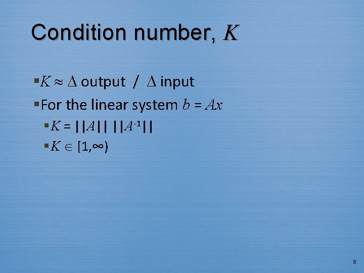
Condition number, K §K output / input §For the linear system b = Ax § K = ||A|| ||A-1|| § K [1, ∞) 8

K for convolved blur § Why is restoration ill-posed for simple blur? § Why not just linearize a blur kernel, and then take the inverse of that matrix? § F = H-1 G § Because H is probably singular § If not, H almost certainly has a large K § So small amounts of noise in G will make the computed F almost meaningless § See the book for great examples 9

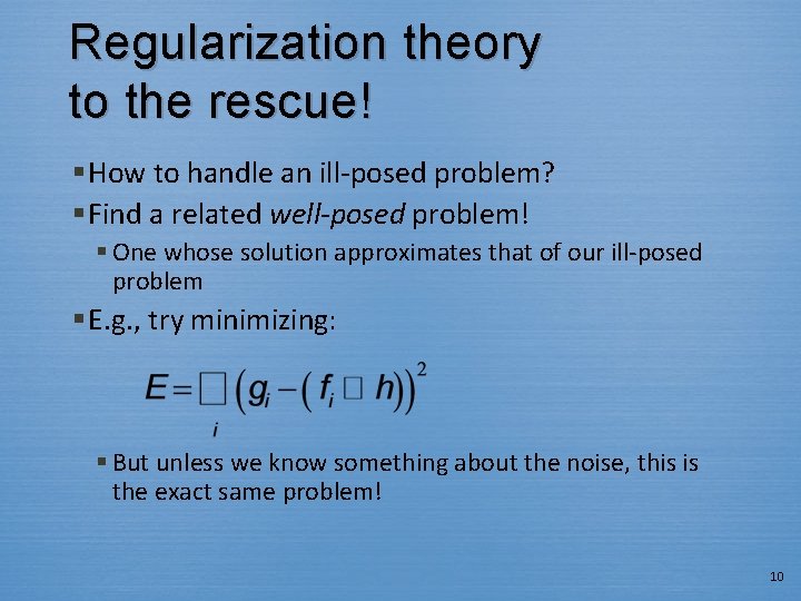
Regularization theory to the rescue! § How to handle an ill-posed problem? § Find a related well-posed problem! § One whose solution approximates that of our ill-posed problem § E. g. , try minimizing: § But unless we know something about the noise, this is the exact same problem! 10

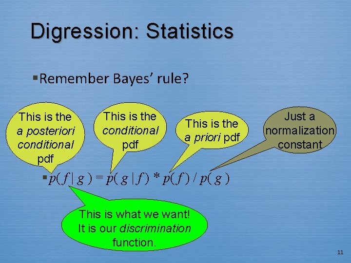
Digression: Statistics §Remember Bayes’ rule? This is the a posteriori conditional pdf This is the a priori pdf Just a normalization constant § p( f | g ) = p( g | f ) * p( f ) / p( g ) This is what we want! It is our discrimination function. 11

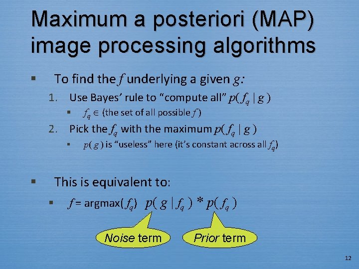
Maximum a posteriori (MAP) image processing algorithms § To find the f underlying a given g: 1. Use Bayes’ rule to “compute all” p( fq | g ) § fq (the set of all possible f ) 2. Pick the fq with the maximum p( fq | g ) § § p( g ) is “useless” here (it’s constant across all fq) This is equivalent to: § f = argmax( fq) p( g | fq ) * p( fq ) Noise term Prior term 12

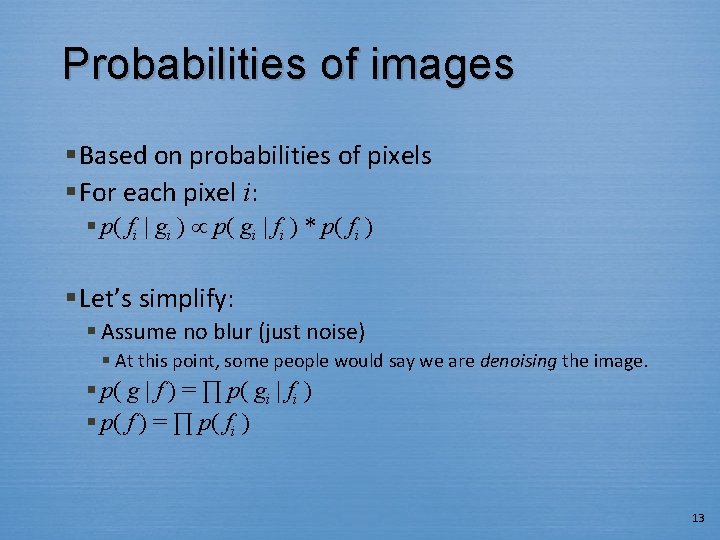
Probabilities of images § Based on probabilities of pixels § For each pixel i: § p( fi | gi ) p( gi | fi ) * p( fi ) § Let’s simplify: § Assume no blur (just noise) § At this point, some people would say we are denoising the image. § p( g | f ) = ∏ p( gi | fi ) § p( f ) = ∏ p( fi ) 13

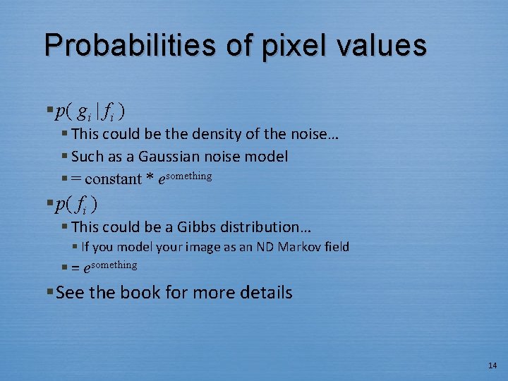
Probabilities of pixel values § p( gi | fi ) § This could be the density of the noise… § Such as a Gaussian noise model § = constant * esomething § p( fi ) § This could be a Gibbs distribution… § If you model your image as an ND Markov field § = esomething § See the book for more details 14

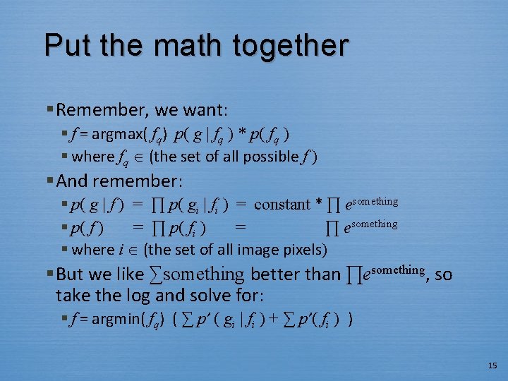
Put the math together § Remember, we want: § f = argmax( fq) p( g | fq ) * p( fq ) § where fq (the set of all possible f ) § And remember: § p( g | f ) = ∏ p( gi | fi ) = constant * ∏ esomething § p( f ) = ∏ p( fi ) = ∏ esomething § where i (the set of all image pixels) § But we like ∑something better than ∏esomething, so take the log and solve for: § f = argmin( fq) ( ∑ p’ ( gi | fi ) + ∑ p’( fi ) ) 15

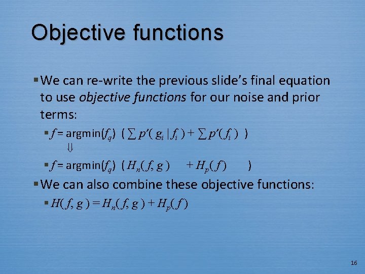
Objective functions § We can re-write the previous slide’s final equation to use objective functions for our noise and prior terms: § f = argmin(fq) ( ∑ p’( gi | fi ) + ∑ p’( fi ) ) § f = argmin(fq) ( Hn( f, g ) + H p( f ) ) § We can also combine these objective functions: § H( f, g ) = Hn( f, g ) + Hp( f ) 16

Purpose of the objective functions § Noise term Hn( f, g ): § If we assume independent, Gaussian noise for each pixel, § We tell the minimization that f should resemble g. § Prior term (a. k. a. regularization term) Hp( f ): § Tells the minimization what properties the image should have § Often, this means brightness that is: § Constant in local areas § Discontinuous at boundaries 17

Minimization is a beast! § Our objective function is not “nice” § It has many local minima § So gradient descent will not do well § We need a more powerful optimizer: § Mean field annealing (MFA) § Approximates simulated annealing § But it’s faster! § It’s also based on the mean field approximation of statistical mechanics 18

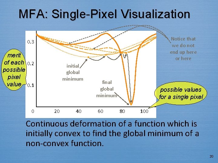
MFA § § MFA is a continuation method So it implements a homotopy § § A homotopy is a continuous deformation of one hyper-surface into another MFA procedure: 1. Distort our complex objective function into a convex hyper-surface (N-surface) § The only minima is now the global minimum 2. Gradually distort the convex N-surface back into our objective function 19

MFA: Single-Pixel Visualization Notice that we do not end up here or here 0. 3 merit of each 0. 2 possible pixel value 0. 1 0 initial global minimum 20 40 final global minimum 60 possible values for a single pixel 80 100 Continuous deformation of a function which is initially convex to find the global minimum of a non-convex function. 20

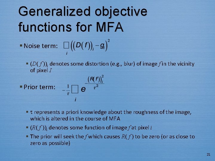
Generalized objective functions for MFA § Noise term: § (D( f ))i denotes some distortion (e. g. , blur) of image f in the vicinity of pixel I § Prior term: § represents a priori knowledge about the roughness of the image, which is altered in the course of MFA § (R( f ))i denotes some function of image f at pixel i § The prior will seek the f which causes R( f ) to be zero (or as close to zero as possible) 21

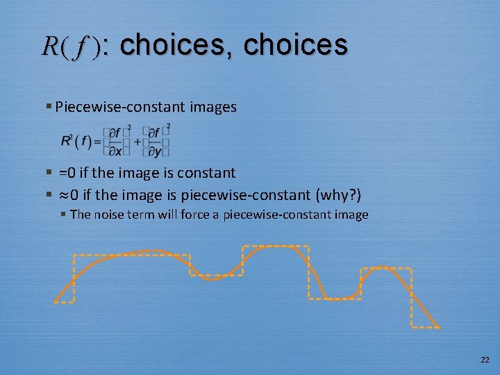
R( f ): choices, choices § Piecewise-constant images § =0 if the image is constant § 0 if the image is piecewise-constant (why? ) § The noise term will force a piecewise-constant image 22

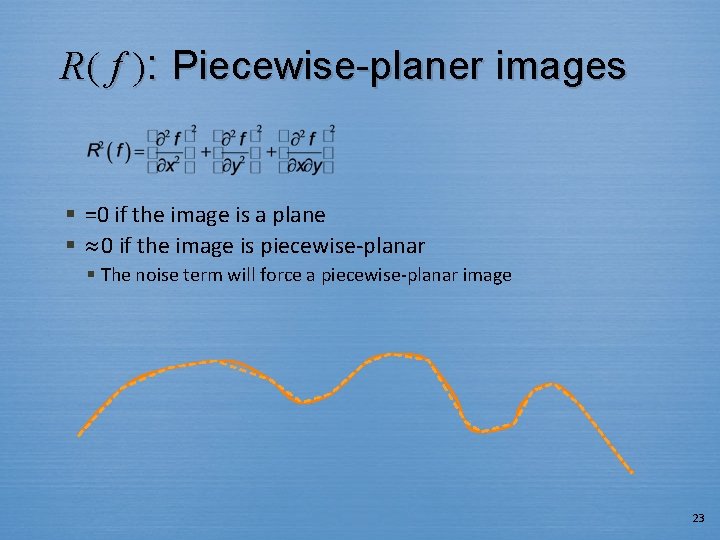
R( f ): Piecewise-planer images § =0 if the image is a plane § 0 if the image is piecewise-planar § The noise term will force a piecewise-planar image 23

Graduated nonconvexity (GNC) § Similar to MFA § Uses a descent method § Reduces a control parameter § Can be derived using MFA as its basis § “Weak membrane” GNC is analogous to piecewiseconstant MFA § But different: § Its objective function treats the presence of edges explicitly § Pixels labeled as edges don’t count in our noise term § So we must explicitly minimize the # of edge pixels 24

Variable conductance diffusion (VCD) §Idea: § Blur an image everywhere, § except at features of interest § such as edges 25

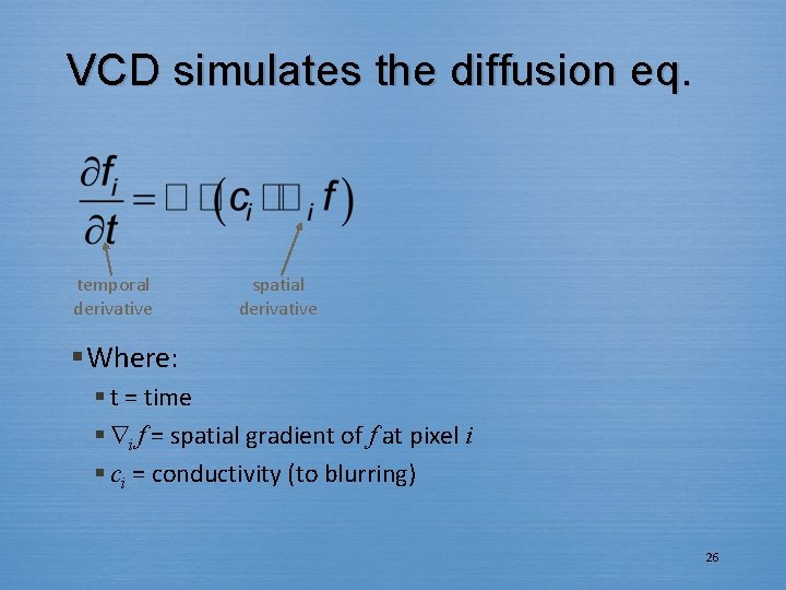
VCD simulates the diffusion eq. temporal derivative spatial derivative § Where: § t = time § i f = spatial gradient of f at pixel i § ci = conductivity (to blurring) 26

Isotropic diffusion §If ci is constant across all pixels: § Isotropic diffusion § Not really VCD § Isotropic diffusion is equivalent to convolution with a Gaussian § The Gaussian’s variance is defined in terms of t and ci 27

VCD § ci is a function of spatial coordinates, parameterized by i § Typically a property of the local image intensities § Can be thought of as a factor by which space is locally compressed § To smooth except at edges: § Let ci be small if i is an edge pixel § Little smoothing occurs because “space is stretched” or “little heat flows” § Let ci be large at all other pixels § More smoothing occurs in the vicinity of pixel i because “space is compressed” or “heat flows easily” 28

VCD § A. K. A. Anisotropic diffusion § With repetition, produces a nearly piecewise uniform result § Like MFA and GNC formulations § Equivalent to MFA w/o a noise term § Edge-oriented VCD: § VCD + diffuse tangential to edges when near edges § Biased Anisotropic diffusion (BAD) § Equivalent to MAP image restoration 29

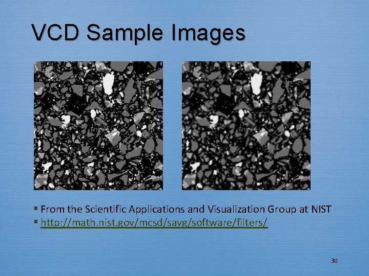
VCD Sample Images § From the Scientific Applications and Visualization Group at NIST § http: //math. nist. gov/mcsd/savg/software/filters/ 30

Congratulations! § You have made it through most of the “introductory” material. § Now we’re ready for the “fun stuff. ” § “Fun stuff” (why we do image analysis): § Segmentation § Registration § Shape Analysis § Etc. 31