Lecture 7 Realtime Digital Signal Processing with the

Lecture 7 Real-time Digital Signal Processing with the TMS 320 C 6 x Dr. Konstantinos Tatas

Outline • Digital Signal Processing Basics – – – ADC and sampling Aliasing Discrete-time signals Digital Filtering FFT Effects of finite fixed-point wordlength • Efficient DSP application implementation on TMS 320 C 6 x processors – FIR filter implementation – IIR filter implementation

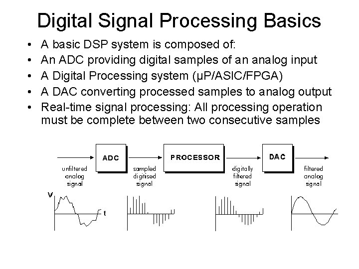
Digital Signal Processing Basics • • • A basic DSP system is composed of: An ADC providing digital samples of an analog input A Digital Processing system (μP/ASIC/FPGA) A DAC converting processed samples to analog output Real-time signal processing: All processing operation must be complete between two consecutive samples

ADC and Sampling • An ADC performs the following: – Sampling – Quantization – Binary Coding • Sampling rate must be at least twice as much as the highest frequency component of the analog input signal

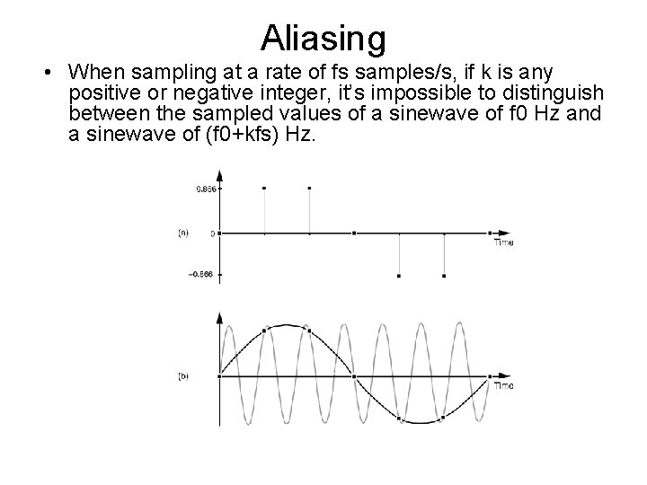
Aliasing • When sampling at a rate of fs samples/s, if k is any positive or negative integer, it’s impossible to distinguish between the sampled values of a sinewave of f 0 Hz and a sinewave of (f 0+kfs) Hz.

Discrete-time signals • A continuous signal input is denoted x(t) • A discrete-time signal is denoted x(n), where n = 0, 1, 2, … • Therefore a discrete time signal is just a collection of samples obtained at regular intervals (sampling frequency)

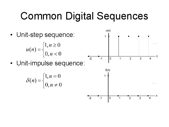
Common Digital Sequences • Unit-step sequence: • Unit-impulse sequence:

The z transform • Discrete equivalent of the Laplace transform

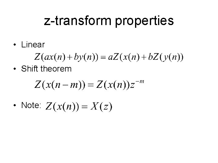
z-transform properties • Linear • Shift theorem • Note:

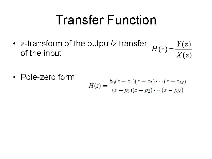
Transfer Function • z-transform of the output/z transfer of the input • Pole-zero form

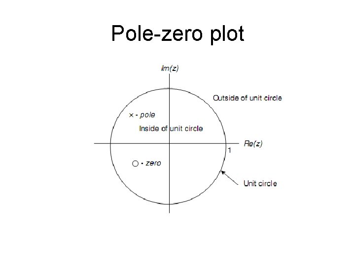
Pole-zero plot

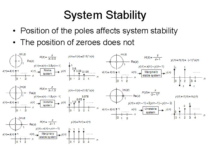
System Stability • Position of the poles affects system stability • The position of zeroes does not

Example 1 • A system is described by the following equation: • y(n)=0. 5 x(n) + 0. 2 x(n-1) + 0. 1 y(n-1) • Plot the system’s transfer function on the z plane • Is the system stable? • Plot the system’s unit step response • Plot the system’s unit impulse response

The Discrete Fourier Transform (DFT) • Discrete equivalent of the continuous Fourier Transform • A mathematical procedure used to determine the harmonic, or frequency, content of a discrete signal sequence •

The Fast Fourier Transform (FFT) • FFT is not an approximation of the DFT, it gives precisely the same result

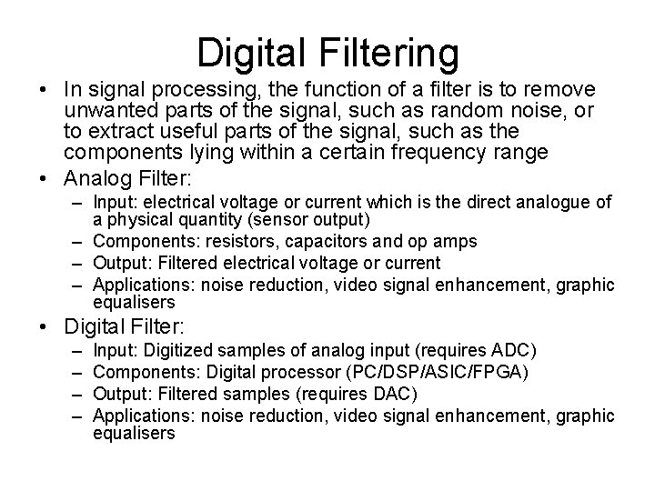
Digital Filtering • In signal processing, the function of a filter is to remove unwanted parts of the signal, such as random noise, or to extract useful parts of the signal, such as the components lying within a certain frequency range • Analog Filter: – Input: electrical voltage or current which is the direct analogue of a physical quantity (sensor output) – Components: resistors, capacitors and op amps – Output: Filtered electrical voltage or current – Applications: noise reduction, video signal enhancement, graphic equalisers • Digital Filter: – – Input: Digitized samples of analog input (requires ADC) Components: Digital processor (PC/DSP/ASIC/FPGA) Output: Filtered samples (requires DAC) Applications: noise reduction, video signal enhancement, graphic equalisers

Averaging Filter

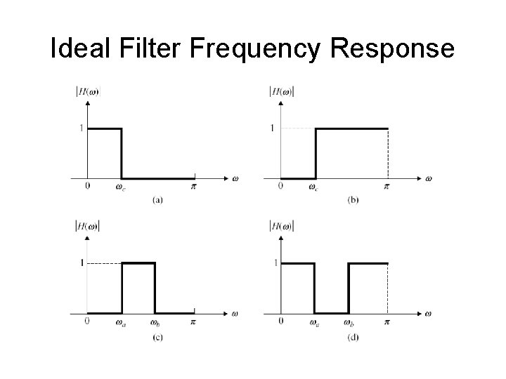
Ideal Filter Frequency Response

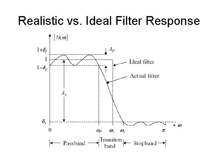
Realistic vs. Ideal Filter Response

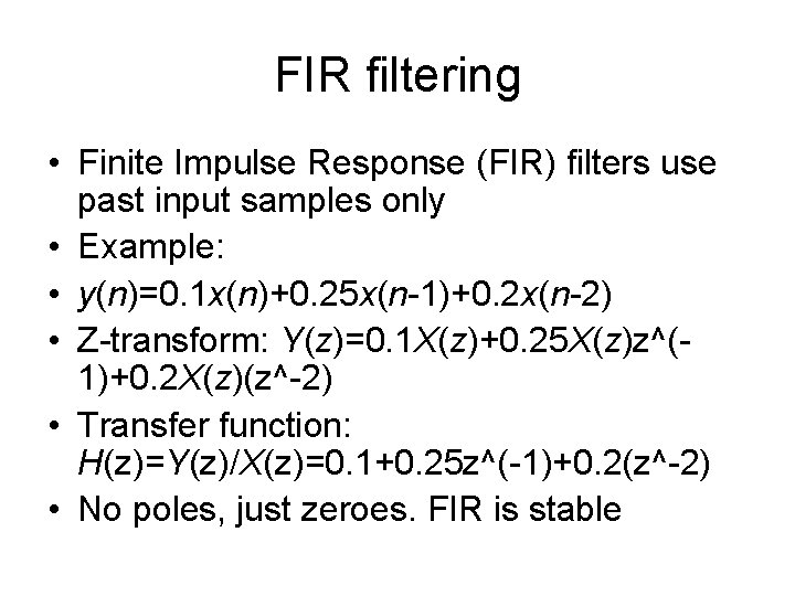
FIR filtering • Finite Impulse Response (FIR) filters use past input samples only • Example: • y(n)=0. 1 x(n)+0. 25 x(n-1)+0. 2 x(n-2) • Z-transform: Y(z)=0. 1 X(z)+0. 25 X(z)z^(1)+0. 2 X(z)(z^-2) • Transfer function: H(z)=Y(z)/X(z)=0. 1+0. 25 z^(-1)+0. 2(z^-2) • No poles, just zeroes. FIR is stable

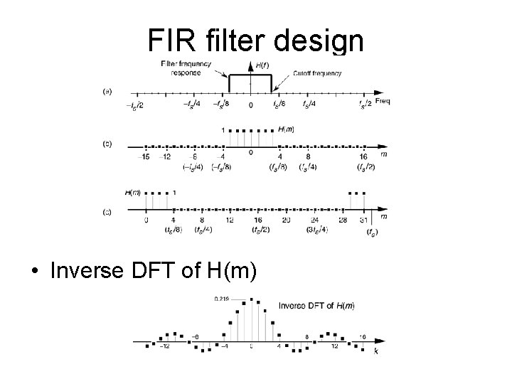
FIR filter design • Inverse DFT of H(m)

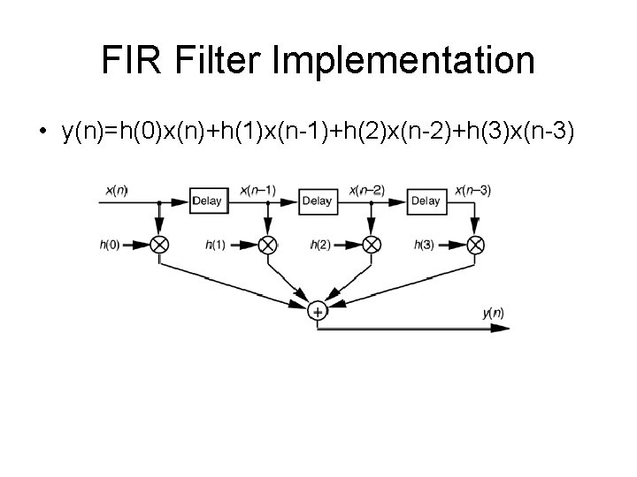
FIR Filter Implementation • y(n)=h(0)x(n)+h(1)x(n-1)+h(2)x(n-2)+h(3)x(n-3)

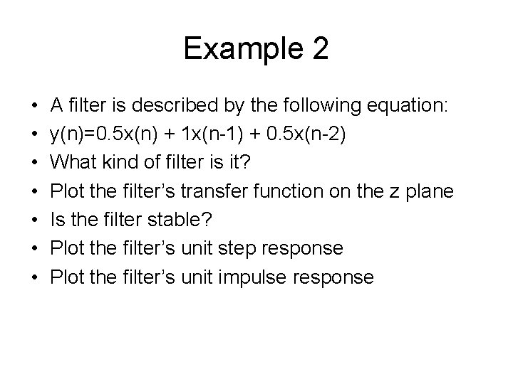
Example 2 • • A filter is described by the following equation: y(n)=0. 5 x(n) + 1 x(n-1) + 0. 5 x(n-2) What kind of filter is it? Plot the filter’s transfer function on the z plane Is the filter stable? Plot the filter’s unit step response Plot the filter’s unit impulse response

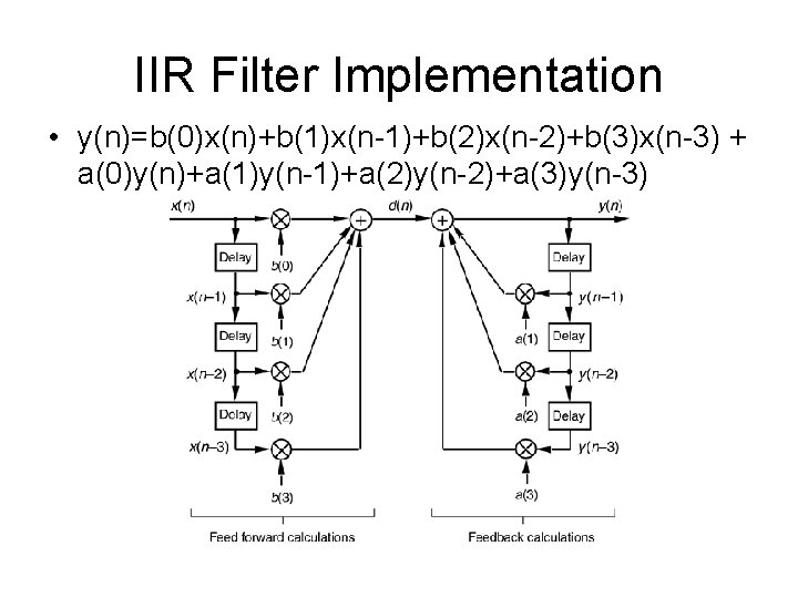
IIR Filtering • Infinite Impulse Response (IIR) filters use past outputs together with past inputs

IIR Filter Implementation • y(n)=b(0)x(n)+b(1)x(n-1)+b(2)x(n-2)+b(3)x(n-3) + a(0)y(n)+a(1)y(n-1)+a(2)y(n-2)+a(3)y(n-3)

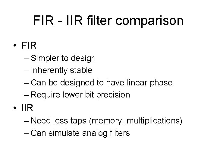
FIR - IIR filter comparison • FIR – Simpler to design – Inherently stable – Can be designed to have linear phase – Require lower bit precision • IIR – Need less taps (memory, multiplications) – Can simulate analog filters

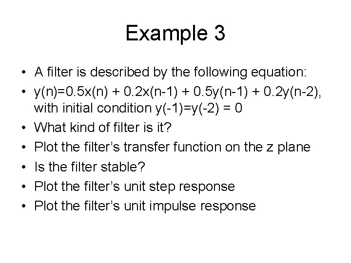
Example 3 • A filter is described by the following equation: • y(n)=0. 5 x(n) + 0. 2 x(n-1) + 0. 5 y(n-1) + 0. 2 y(n-2), with initial condition y(-1)=y(-2) = 0 • What kind of filter is it? • Plot the filter’s transfer function on the z plane • Is the filter stable? • Plot the filter’s unit step response • Plot the filter’s unit impulse response

Software and Hardware Implementation of FIR filters

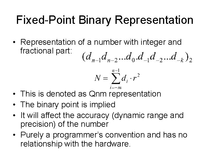
Fixed-Point Binary Representation • Representation of a number with integer and fractional part: • This is denoted as Qnm representation • The binary point is implied • It will affect the accuracy (dynamic range and precision) of the number • Purely a programmer’s convention and has no relationship with the hardware.

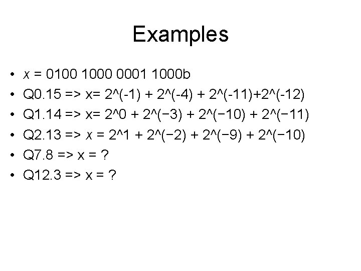
Examples • • • x = 0100 1000 0001 1000 b Q 0. 15 => x= 2^(-1) + 2^(-4) + 2^(-11)+2^(-12) Q 1. 14 => x= 2^0 + 2^(− 3) + 2^(− 10) + 2^(− 11) Q 2. 13 => x = 2^1 + 2^(− 2) + 2^(− 9) + 2^(− 10) Q 7. 8 => x = ? Q 12. 3 => x = ?

EFFECTS OF FINITE FIXEDPOINT BINARY WORD LENGTH • Quantization Errors – ADC – Coefficients • Truncation • Rounding • Data Overflow

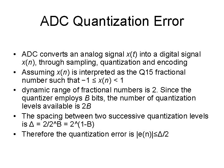
ADC Quantization Error • ADC converts an analog signal x(t) into a digital signal x(n), through sampling, quantization and encoding • Assuming x(n) is interpreted as the Q 15 fractional number such that − 1 ≤ x(n) < 1 • dynamic range of fractional numbers is 2. Since the quantizer employs B bits, the number of quantization levels available is 2 B • The spacing between two successive quantization levels is Δ = 2/2^B = 2^(1 -B) • Therefore the quantization error is |e(n)|≤Δ/2

Coefficient Quantization Error • Effects on FIR filters – Location of zeroes changes – Therefore, frequency response changes • Effects on IIR filters – Location of poles and zeroes change – Could move poles outside of unit circle, leading to unstable implementations

Roundoff error

Overflow error • signals and coefficients normalized in the range of − 1 to 1 for fixed-point arithmetic, the sum of two B-bit numbers may fall outside the range of − 1 to 1. • Severely distorts the signal • Overflow handling – Saturation arithmetic • “Clips” the signal, although better than overflow • Should only be used to guarantee no overflow, but should not be the only solution – Scaling of signals and coefficients

Coefficient representation • Fractional 2’s complement (Q) representation is used • To avoid overflow, often scaling down by a power of two factor (S) (right shift) is used. • The scaling factor is given by the equation: S=Imax(|h(0)|+|h(1)|+|h(2)|+…) • Furthermore, filter coefficient larger than 1, cause overflow and are scaled down further by a factor B, in order to be less than 1

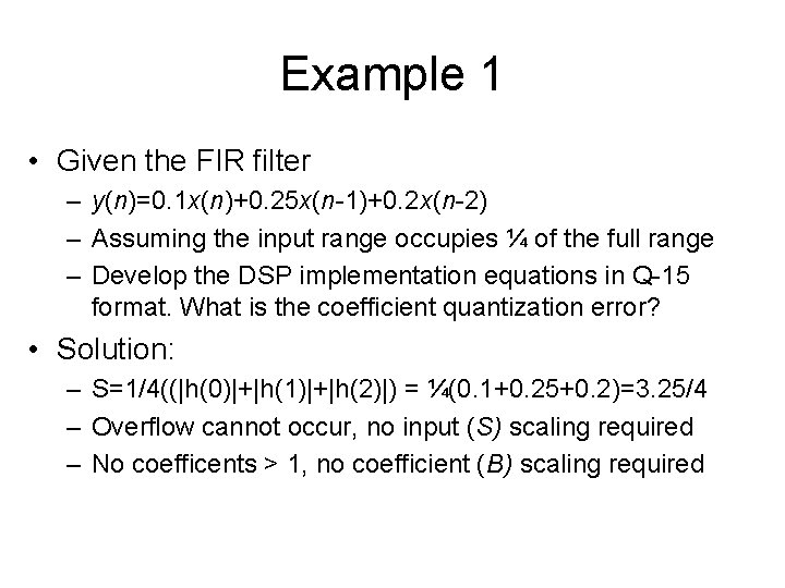
Example 1 • Given the FIR filter – y(n)=0. 1 x(n)+0. 25 x(n-1)+0. 2 x(n-2) – Assuming the input range occupies ¼ of the full range – Develop the DSP implementation equations in Q-15 format. What is the coefficient quantization error? • Solution: – S=1/4((|h(0)|+|h(1)|+|h(2)|) = ¼(0. 1+0. 25+0. 2)=3. 25/4 – Overflow cannot occur, no input (S) scaling required – No coefficents > 1, no coefficient (B) scaling required

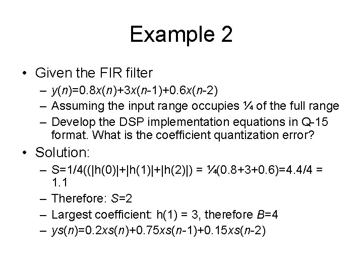
Example 2 • Given the FIR filter – y(n)=0. 8 x(n)+3 x(n-1)+0. 6 x(n-2) – Assuming the input range occupies ¼ of the full range – Develop the DSP implementation equations in Q-15 format. What is the coefficient quantization error? • Solution: – S=1/4((|h(0)|+|h(1)|+|h(2)|) = ¼(0. 8+3+0. 6)=4. 4/4 = 1. 1 – Therefore: S=2 – Largest coefficient: h(1) = 3, therefore B=4 – ys(n)=0. 2 xs(n)+0. 75 xs(n-1)+0. 15 xs(n-2)

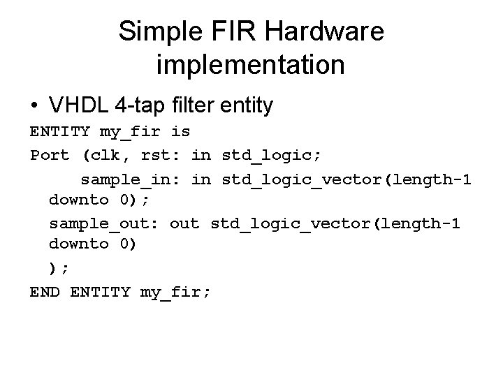
Simple FIR Hardware implementation • VHDL 4 -tap filter entity ENTITY my_fir is Port (clk, rst: in std_logic; sample_in: in std_logic_vector(length-1 downto 0); sample_out: out std_logic_vector(length-1 downto 0) ); END ENTITY my_fir;

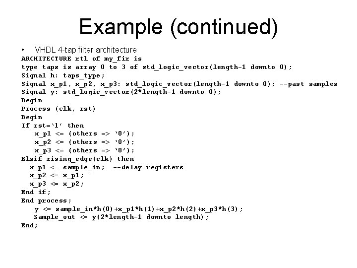
Example (continued) • VHDL 4 -tap filter architecture ARCHITECTURE rtl of my_fir is type taps is array 0 to 3 of std_logic_vector(length-1 downto 0); Signal h: taps_type; Signal x_p 1, x_p 2, x_p 3: std_logic_vector(length-1 downto 0); --past samples Signal y: std_logic_vector(2*length-1 downto 0); Begin Process (clk, rst) Begin If rst=‘ 1’ then x_p 1 <= (others => ‘ 0’); x_p 2 <= (others => ‘ 0’); x_p 3 <= (others => ‘ 0’); Elsif rising_edge(clk) then x_p 1 <= sample_in; --delay registers x_p 2 <= x_p 1; x_p 3 <= x_p 2; End if; End process; y <= sample_in*h(0)+x_p 1*h(1)+x_p 2*h(2)+x_p 3*h(3); Sample_out <= y(2*length-1 downto length); End;

FIR Software Implementation int yn=0; short xdly[N+1]; //filter output initialization //input delay samples array interrupt void c_int 11() //ISR { short i; yn=0; short h[N] = { //coefficients }; xdly[0]=input_sample(); for (i=0; i<N; i++) yn += (h[i]*xdly[i]); for (i=N-1; i>0; i--) xdly[i] = xdly[i-1]; output_sample(yn >> 15); //filter output return; //return from ISR }

IIR C implementation int yn=0; short xdly[N+1]; Short ydly[M]; //filter output initialization //input delay samples array //output delay array interrupt void c_int 11() //ISR { short i; yn=0; short a[N] = { //coefficients }; short b[M] = { //coefficients }; xdly[0]=input_sample(); for (i=0; i<N; i++) yn += (a[i]*xdly[i]); for (i=0; i<M; i++) yn += (b[i]*ydly[i]); for (i=N-1; i>0; i--) xdly[i] = xdly[i-1]; ydly[0] = yn >> 15; for (i=M-1; i>0; i--) ydly[i] = ydly[i-1]; output_sample(yn >> 15); //filter output return; //return from ISR }