Lecture 7 PRAM Algorithm Parallel Prefix Parallel Computing

Lecture 7 PRAM Algorithm: Parallel Prefix Parallel Computing Fall 2008 1

Parallel Operations with Multiple Outputs – Parallel Prefix n n n Problem definition: Given a set of n values x 0, x 1, . . . , xn− 1 and an associative operator, say +, the parallel prefix problem is to compute the following n results/“sums”. 0: x 0, 1: x 0 + x 1, 2: x 0 + x 1 + x 2, . . . n − 1: x 0 + x 1 +. . . + xn− 1. Parallel prefix is also called prefix sums or scan. It has many uses in parallel computing such as in load-balancing the work assigned to processors and compacting data structures such as arrays. We shall prove that computing ALL THE SUMS is no more difficult that computing the single sum x 0 +. . . xn− 1. 2

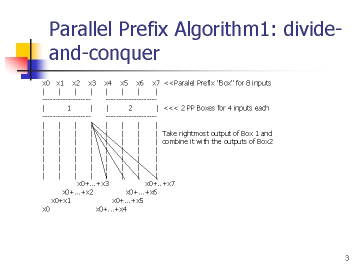
Parallel Prefix Algorithm 1: divideand-conquer x 0 x 1 x 2 x 3 x 4 x 5 x 6 x 7 <<Paralel Prefix "Box" for 8 inputs | | | | -------------------| 1 | | 2 | <<< 2 PP Boxes for 4 inputs each -------------------| | | | Take rightmost output of Box 1 and | | | | combine it with the outputs of Box 2 | | | | | | | | x 0+. . . +x 3 x 0+. . +x 7 x 0+. . . +x 2 x 0+. . . +x 6 x 0+x 1 x 0+. . . +x 5 x 0+. . . +x 4 3

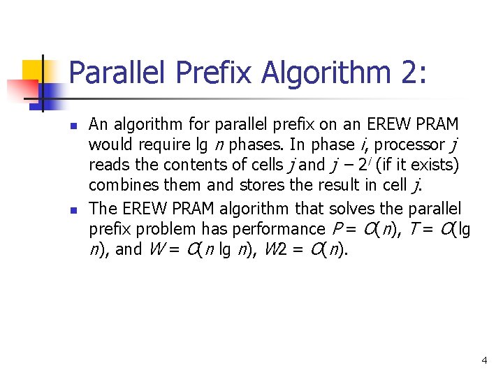
Parallel Prefix Algorithm 2: n n An algorithm for parallel prefix on an EREW PRAM would require lg n phases. In phase i, processor j reads the contents of cells j and j − 2 i (if it exists) combines them and stores the result in cell j. The EREW PRAM algorithm that solves the parallel prefix problem has performance P = O(n), T = O(lg n), and W = O(n lg n), W 2 = O(n). 4

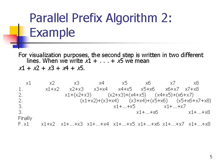
Parallel Prefix Algorithm 2: Example For visualization purposes, the second step is written in two different lines. When we write x 1 +. . . + x 5 we mean x 1 + x 2 + x 3 + x 4 + x 5. x 1 1. 2. 2. 3. 3. Finally F. x 1 x 2 x 1+x 2 x 3 x 4 x 5 x 6 x 7 x 8 x 2+x 3 x 3+x 4 x 4+x 5 x 5+x 6 x 6+x 7 x 7+x 8 x 1+(x 2+x 3)+(x 4+x 5)+(x 6+x 7) (x 1+x 2)+(x 3+x 4)+(x 5+x 6) (x 5+x 6+x 7+x 8) x 1+. . . +x 5 x 1+. . . +x 7 x 1+. . . +x 6 x 1+. . . +x 8 x 1+. . . +x 3 x 1+. . . +x 4 x 1+. . . +x 5 x 1+. . . +x 6 x 1+. . . +x 7 x 1+. . . +x 8 5

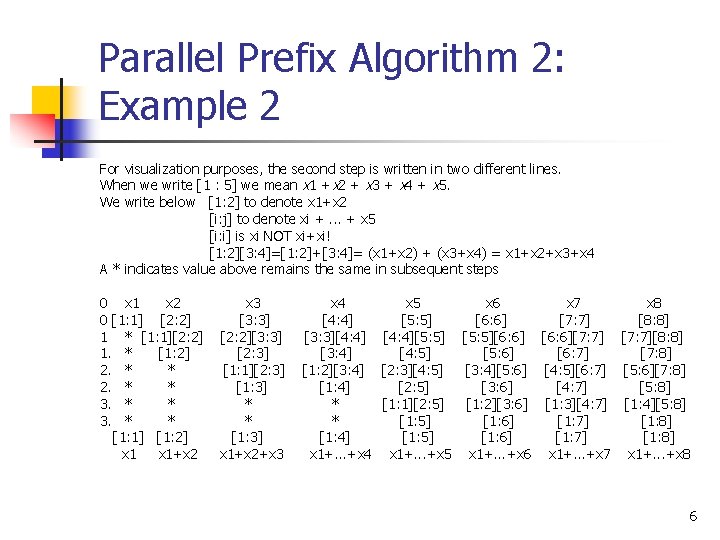
Parallel Prefix Algorithm 2: Example 2 For visualization purposes, the second step is written in two different lines. When we write [1 : 5] we mean x 1 +x 2 + x 3 + x 4 + x 5. We write below [1: 2] to denote x 1+x 2 [i: j] to denote xi +. . . + x 5 [i: i] is xi NOT xi+xi! [1: 2][3: 4]=[1: 2]+[3: 4]= (x 1+x 2) + (x 3+x 4) = x 1+x 2+x 3+x 4 A * indicates value above remains the same in subsequent steps 0 x 1 x 2 0 [1: 1] [2: 2] 1 * [1: 1][2: 2] 1. * [1: 2] 2. * * 3. * * [1: 1] [1: 2] x 1+x 2 x 3 [3: 3] [2: 2][3: 3] [2: 3] [1: 1][2: 3] [1: 3] * * [1: 3] x 1+x 2+x 3 x 4 x 5 x 6 x 7 x 8 [4: 4] [5: 5] [6: 6] [7: 7] [8: 8] [3: 3][4: 4][5: 5][6: 6][7: 7][8: 8] [3: 4] [4: 5] [5: 6] [6: 7] [7: 8] [1: 2][3: 4] [2: 3][4: 5] [3: 4][5: 6] [4: 5][6: 7] [5: 6][7: 8] [1: 4] [2: 5] [3: 6] [4: 7] [5: 8] * [1: 1][2: 5] [1: 2][3: 6] [1: 3][4: 7] [1: 4][5: 8] * [1: 5] [1: 6] [1: 7] [1: 8] [1: 4] [1: 5] [1: 6] [1: 7] [1: 8] x 1+. . . +x 4 x 1+. . . +x 5 x 1+. . . +x 6 x 1+. . . +x 7 x 1+. . . +x 8 6

Parallel Prefix Algorithm 2: // We write below[1: 2] to denote X[1]+X[2] // [i: j] to denote X[i]+X[i+1]+. . . +X[j] // [i: i] is X[i] NOT X[i]+X[i] // [1: 2][3: 4]=[1: 2]+[3: 4]= (X[1]+X[2])+(X[3]+X[4])=X[1]+X[2]+X[3]+X[4] // Input : M[j]= X[j]=[j: j] for j=1, . . . , n. // Output: M[j]= X[1]+. . . +X[j] = [1: j] for j=1, . . . , n. Parallel. Prefix(n) 1. i=1; // At this step M[j]= [j: j]=[j+1 -2**(i-1): j] 2. while (i < n ) { 3. j=pid(); 4. if (j-2**(i-1) >0 ) { 5. a=M[j]; // Before this step. M[j] = [j+1 -2**(i-1): j] 6. b=M[j-2**(i-1)]; // Before this step. M[j-2**(i-1)]= [j-2**(i-1)+1 -2**(i-1): j-2**(i-1)] 7. M[j]=a+b; // After this step M[j]= M[j]+M[j-2**(i-1)]=[j-2**(i-1)+1 -2**(i-1): j-2**(i 1)] // [j+1 -2**(i-1): j] = [j-2**(i-1)+1 -2**(i-1): j]=[j+1 -2**i: j] 8. } 9. i=i*2; } At step 5, memory location j − 2 i− 1 is read provided that j − 2 i− 1 ≥ 1. This is true for all times i ≤ tj = lg(j − 1) + 1. For i > tj the test of line 4 fails and lines 5 -8 are not executed. 7

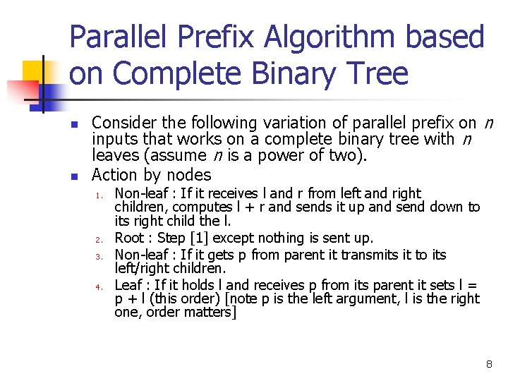
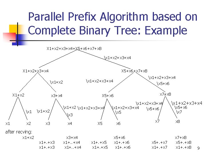
Parallel Prefix Algorithm based on Complete Binary Tree n n Consider the following variation of parallel prefix on n inputs that works on a complete binary tree with n leaves (assume n is a power of two). Action by nodes 1. 2. 3. 4. Non-leaf : If it receives l and r from left and right children, computes l + r and sends it up and send down to its right child the l. Root : Step [1] except nothing is sent up. Non-leaf : If it gets p from parent it transmits it to its left/right children. Leaf : If it holds l and receives p from its parent it sets l = p + l (this order) [note p is the left argument, l is the right one, order matters] 8

Parallel Prefix Algorithm based on Complete Binary Tree: Example X 1+x 2+x 3+x 4+X 5+x 6+x 7+x 8 x 1+x 2+x 3+x 4 X 1+x 2 x 1 x 1+x 2 x 3 X 5+x 6+x 7+x 8 x 1+x 2+x 3+x 4 X 5+x 6 x 1+x 2+x 3+x 4 x 3 x 4 X 5 x 1+x 2+x 3+x 4 x 5+x 6 x 7+x 8 x 1+x 2+x 3+x 4 x 5+x 6 x 5 x 6 x 7 x 1+x 2+x 3+x 4 x 5+x 6 x 7 x 8 after recving: x 1+x 2 x 1+. +x 3 x 3+x 4 x 1+. +x 5 x 5+x 6 x 1+. +x 6 x 5+. +x 7 x 1+. +x 7 x 7+x 8 x 5+. +x 8 x 1+. +x 8 9

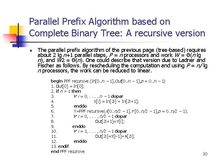
Parallel Prefix Algorithm based on Complete Binary Tree: A recursive version n The parallel prefix algorithm of the previous page (tree-based) requires about 2 lg n+1 parallel steps, P = n processors and work W = Θ(n lg n), and W 2 = Θ(n). One could describe that version due to Ladner and Fischer as follows. By rescheduling the computation and using P = n/ lg n processors, the work can be reduced to linear. begin PPF recursive (In[0. . n − 1], Out[0. . n − 1], p = 0. . n − 1) 1. Out[0] = In[0]; 2. if n > 1 then 3. ∀ i = 0, . . . , n − 1 dopar 4. X[i] = In[2 i] + In[2 i+1]; 5. enddo 6. Y=PPF recursive(X[0. . n/2 − 1], Y [0. . n/2 − 1], p = 0. . n/2 − 1); 7. ∀ i = 0, . . . , n/2 − 1 dopar 8. Out[2 i+1]=Y[i]; 9. enddo 10. ∀ i = 1, . . . , n/2 − 1 dopar 11. Out[2 i]=Y[i-1]+A[2 i]; 12. enddo 13. endif end PPF recursive 10

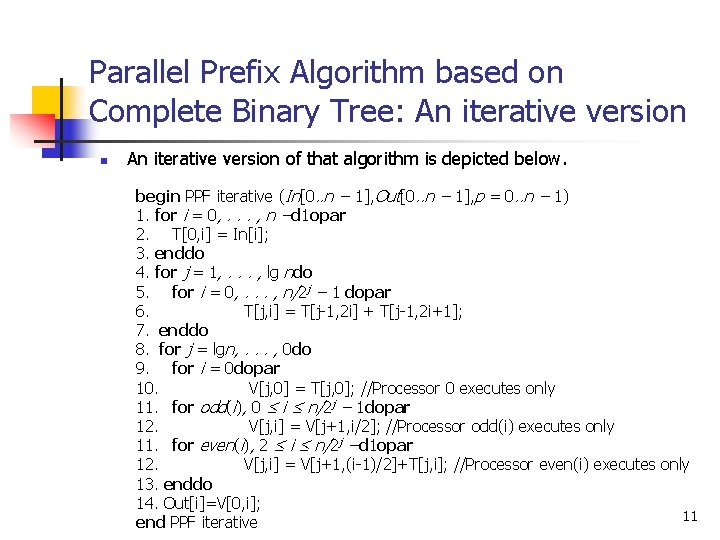
Parallel Prefix Algorithm based on Complete Binary Tree: An iterative version n An iterative version of that algorithm is depicted below. begin PPF iterative (In[0. . n − 1], Out[0. . n − 1], p = 0. . n − 1) 1. for i = 0, . . . , n −d 1 opar 2. T[0, i] = In[i]; 3. enddo 4. for j = 1, . . . , lg ndo 5. for i = 0, . . . , n/2 j − 1 dopar 6. T[j, i] = T[j-1, 2 i] + T[j-1, 2 i+1]; 7. enddo 8. for j = lgn, . . . , 0 do 9. for i = 0 dopar 10. V[j, 0] = T[j, 0]; //Processor 0 executes only 11. for odd(i), 0 ≤ i ≤ n/2 j − 1 dopar 12. V[j, i] = V[j+1, i/2]; //Processor odd(i) executes only 11. for even(i), 2 ≤ i ≤ n/2 j −d 1 opar 12. V[j, i] = V[j+1, (i-1)/2]+T[j, i]; //Processor even(i) executes only 13. enddo 14. Out[i]=V[0, i]; 11 end PPF iterative

End Thank you! 12