Lecture 7 5 1 5 2 Discrete Probability

Lecture 7 5. 1 5. 2 Discrete Probability

5. 1 Probabilities • Important in study of complexity of algorithms. • Modeling the uncertain world: information, data. • Applications in error-correcting coding, data compression, data restoration, medical expert systems, search engines, etc. • Modern AI deals with uncertainty in the world (was my measurement correct, were my assumptions correct). Probability theory is the answer to that. • Developed in the context of gambling.

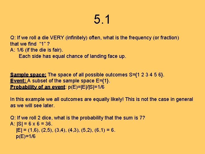
5. 1 Q: If we roll a die VERY (infinitely) often, what is the frequency (or fraction) that we find “ 1” ? A: 1/6 (if the die is fair). Each side has equal chance of landing face up. Sample space: The space of all possible outcomes S={1 2 3 4 5 6}. Event: A subset of the sample space E={1}. Probability of an event: p(E)=|E|/|S|=1/6 In this example we all outcomes are equally likely! This is not the case in general as we will see later. Q: If we roll 2 dice, what is the probability that the sum is 7? A: |S| = 6 x 6 = 36. |E| = (1, 6), (2, 5), (3, 4), (4, 3), (5, 2), (6, 1) = 6. p(E)=1/6

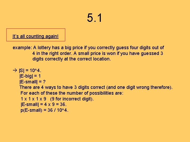
5. 1 It’s all counting again! example: A lottery has a big price if you correctly guess four digits out of 4 in the right order. A small price is won if you have guessed 3 digits correctly at the correct location. |S| = 10^4. |E-big| = 1 |E-small| = ? There are 4 ways to have 3 digits correct (and one digit wrong therefore). For each of these the number of possibilities are: 1 x 1 x 9 (9 for incorrect digit). |E-small| = 4 x 9 = 36. p(E-small) = 36 / 10^4.

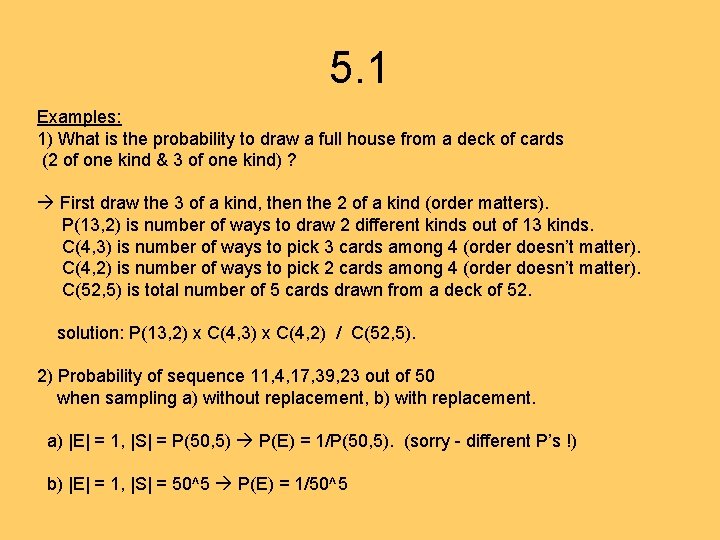
5. 1 Examples: 1) What is the probability to draw a full house from a deck of cards (2 of one kind & 3 of one kind) ? First draw the 3 of a kind, then the 2 of a kind (order matters). P(13, 2) is number of ways to draw 2 different kinds out of 13 kinds. C(4, 3) is number of ways to pick 3 cards among 4 (order doesn’t matter). C(4, 2) is number of ways to pick 2 cards among 4 (order doesn’t matter). C(52, 5) is total number of 5 cards drawn from a deck of 52. solution: P(13, 2) x C(4, 3) x C(4, 2) / C(52, 5). 2) Probability of sequence 11, 4, 17, 39, 23 out of 50 when sampling a) without replacement, b) with replacement. a) |E| = 1, |S| = P(50, 5) P(E) = 1/P(50, 5). (sorry - different P’s !) b) |E| = 1, |S| = 50^5 P(E) = 1/50^5

5. 1 Theorem: Let denote the complement of E. Then: Proof: | | = |S|-|E|. = |S| - |E| / |S| = 1 – p(E). Example: We generate a bit-string of length 10. What is the probability that at least one bit has a 0? E = large and hard to enumerate. = small: no zeros in the bit-string! Only one possibility. p(E) = 1 - = 1 – 1 / 2^10 = 1023/1024.

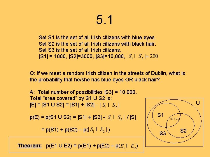
5. 1 Set S 1 is the set of all Irish citizens with blue eyes. Set S 2 is the set of all Irish citizens with black hair. Set S 3 is the set of all Irish citizens. |S 1| = 1000, |S 2|=3000, |S 3|=10, 000, Q: If we meet a random Irish citizen in the streets of Dublin, what is the probability that he/she has blue eyes OR black hair? A: Total number of possibilities |S 3| = 10, 000. Total “area covered” by S 1 U S 2 is: |E| = |S 1 U S 2| = |S 1| + |S 2| p(E) = p(S 1 U S 2) = |S 1| + |S 2| = p(S 1) + p(S 2) – p( S 1 / |S| ) Theorem: p(E 1 U E 2) = p(E 1) + p(E 2) – p( U S 3 ) S 2

5. 1 A famous example: You participate in a game where there are 3 doors with only one hiding a big price. You pick a door. The game show host (who knows where the price is), opens another empty door and offers you to switch. Should you? You don’t switch: You have probability 1/3 to pick the correct door. If you don’t switch that doesn’t change (imagine doing the experiment a million times with this strategy). You switch: If you got the correct door (prob. 1/3) and you switch you lost. If you got the wrong door (prob. 2/3) and you switch you win!

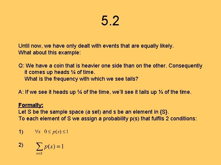
5. 2 Until now, we have only dealt with events that are equally likely. What about this example: Q: We have a coin that is heavier one side than on the other. Consequently it comes up heads ¾ of time. What is the frequency with which we see tails? A: If we see it heads up ¾ of the time, we’ll see it tails up ¼ of the time. Formally: Let S be the sample space (a set) and s be an element in {S}. To each element of S we assign a probability p(s) that fulfils 2 conditions: 1) 2)

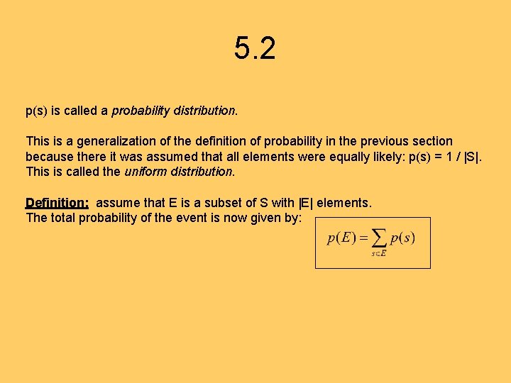
5. 2 p(s) is called a probability distribution. This is a generalization of the definition of probability in the previous section because there it was assumed that all elements were equally likely: p(s) = 1 / |S|. This is called the uniform distribution. Definition: assume that E is a subset of S with |E| elements. The total probability of the event is now given by:

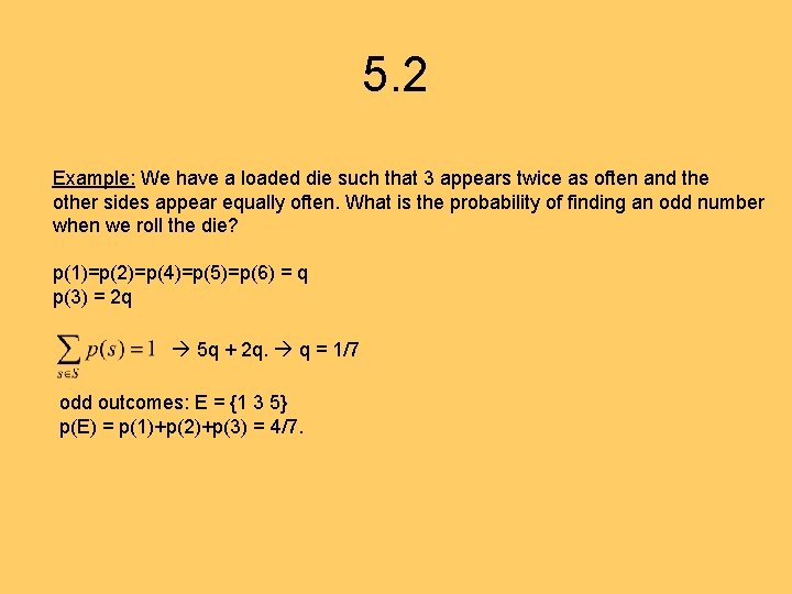
5. 2 Example: We have a loaded die such that 3 appears twice as often and the other sides appear equally often. What is the probability of finding an odd number when we roll the die? p(1)=p(2)=p(4)=p(5)=p(6) = q p(3) = 2 q 5 q + 2 q. q = 1/7 odd outcomes: E = {1 3 5} p(E) = p(1)+p(2)+p(3) = 4/7.

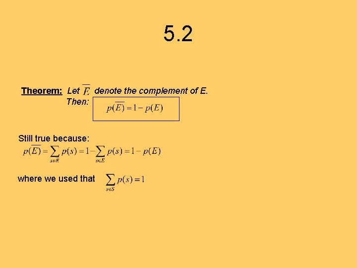
5. 2 Theorem: Let denote the complement of E. Then: Still true because: where we used that

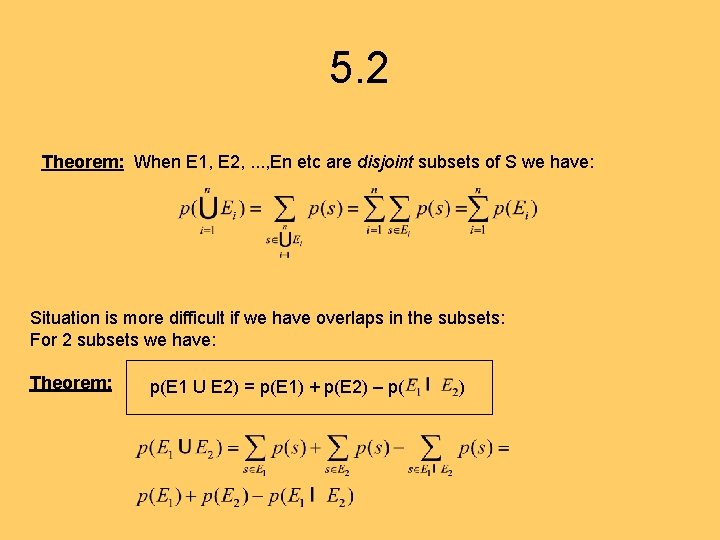
5. 2 Theorem: When E 1, E 2, . . . , En etc are disjoint subsets of S we have: Situation is more difficult if we have overlaps in the subsets: For 2 subsets we have: Theorem: p(E 1 U E 2) = p(E 1) + p(E 2) – p( )

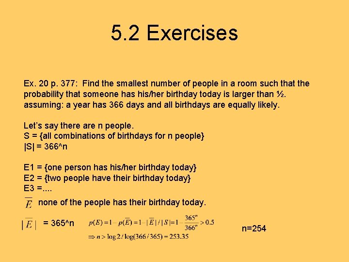
5. 2 Exercises Ex. 20 p. 377: Find the smallest number of people in a room such that the probability that someone has his/her birthday today is larger than ½. assuming: a year has 366 days and all birthdays are equally likely. Let’s say there are n people. S = {all combinations of birthdays for n people} |S| = 366^n E 1 = {one person has his/her birthday today} E 2 = {two people have their birthday today} E 3 =. . none of the people has their birthday today. = 365^n n=254

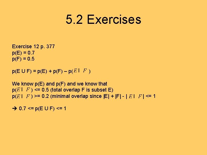
5. 2 Exercises Exercise 12 p. 377 p(E) = 0. 7 p(F) = 0. 5 p(E U F) = p(E) + p(F) – p( ) We know p(E) and p(F) and we know that p( ) <= 0. 5 (total overlap F is subset E) p( ) >= 0. 2 (minimal overlap since |E| + |F| - | 0. 7 <= p(E U F) <= 1 | <= 1