Lecture 6 Supervised Learning Unsupervised Learning Learning From

Lecture 6 Supervised Learning

Unsupervised Learning • Learning From Unlabeled Data • Clustering, Correlation, PCA • Identify relationships between the features

Supervised Learning • Learning From Labeled Data • Neural Networks, Support Vector Machines, Decision Trees • Identify relationships between the features and the categories

Supervised Learning • Given: – Examples whose feature values are known and – Whose categories are known • Do: – Predict the categories of examples whose feature values are known but whose categories are not

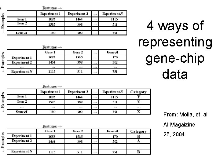
4 ways of representing gene-chip data From: Molla, et. a. I AI Magaizine 25, 2004

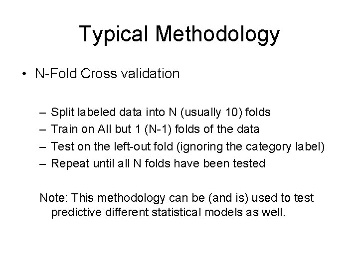
Typical Methodology • N-Fold Cross validation – – Split labeled data into N (usually 10) folds Train on All but 1 (N-1) folds of the data Test on the left-out fold (ignoring the category label) Repeat until all N folds have been tested Note: This methodology can be (and is) used to test predictive different statistical models as well.

Example: Probe Picking

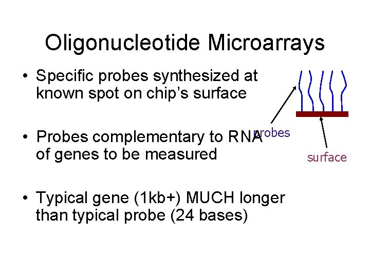
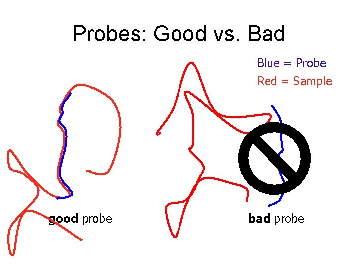
Oligonucleotide Microarrays • Specific probes synthesized at known spot on chip’s surface probes • Probes complementary to RNA of genes to be measured • Typical gene (1 kb+) MUCH longer than typical probe (24 bases) surface

Probes: Good vs. Bad Blue = Probe Red = Sample good probe bad probe

Probe-Picking Method Needed • Hybridization characteristics differ between probes • Probe set represents very small subset of gene • Accurate measurement of expression requires good probe set

Related Work • Use known hybridization characteristics Lockhardt et al. 1996 • Melting point (Tm) predictions Kurata and Suyama 1999 Li and Stormo 2001 • Stable secondary structure Kurata and Suyama 1999

Our Approach • Apply established machine-learning algorithms – Train on categorized examples – Test on examples with category hidden • Choose features to represent probes • Categorize probes as good or bad

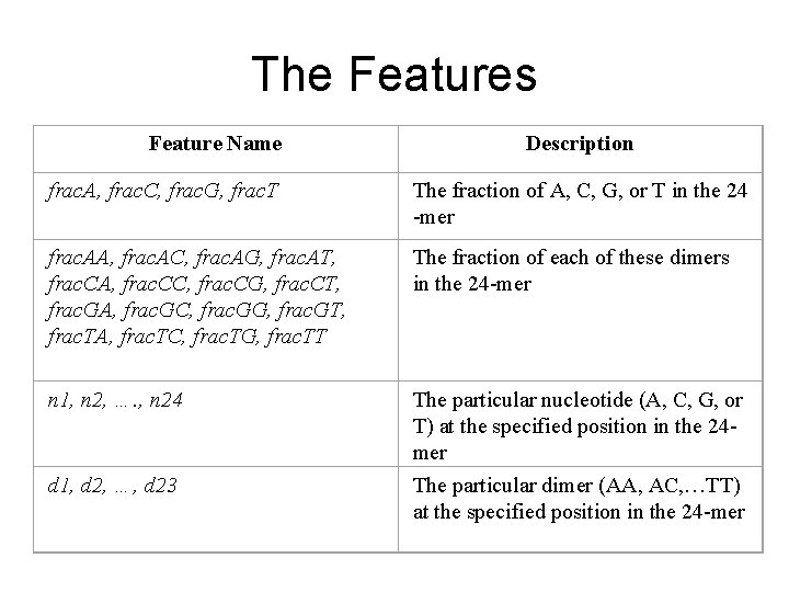
The Features Feature Name Description frac. A, frac. C, frac. G, frac. T The fraction of A, C, G, or T in the 24 -mer frac. AA, frac. AC, frac. AG, frac. AT, frac. CA, frac. CC, frac. CG, frac. CT, frac. GA, frac. GC, frac. GG, frac. GT, frac. TA, frac. TC, frac. TG, frac. TT The fraction of each of these dimers in the 24 -mer n 1, n 2, …. , n 24 The particular nucleotide (A, C, G, or T) at the specified position in the 24 mer The particular dimer (AA, AC, …TT) at the specified position in the 24 -mer d 1, d 2, …, d 23

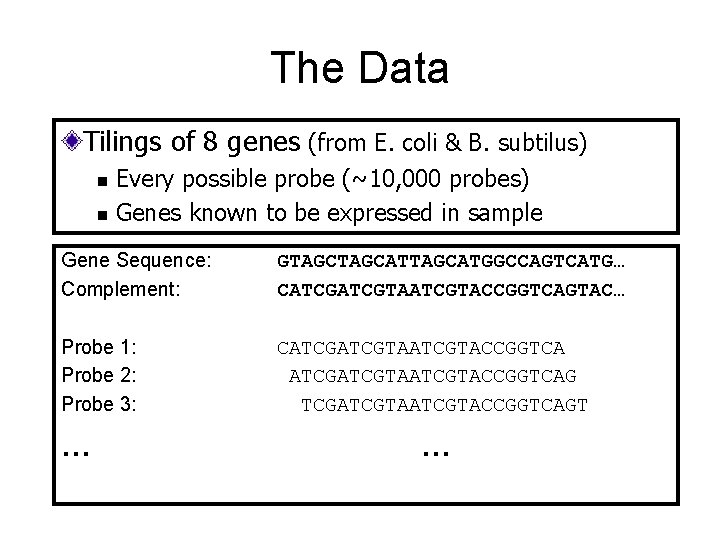
The Data Tilings of 8 genes (from E. coli & B. subtilus) n n Every possible probe (~10, 000 probes) Genes known to be expressed in sample Gene Sequence: Complement: GTAGCATTAGCATGGCCAGTCATG… CATCGTAATCGTACCGGTCAGTAC… Probe 1: Probe 2: Probe 3: CATCGTAATCGTACCGGTCAG TCGATCGTACCGGTCAGT … …

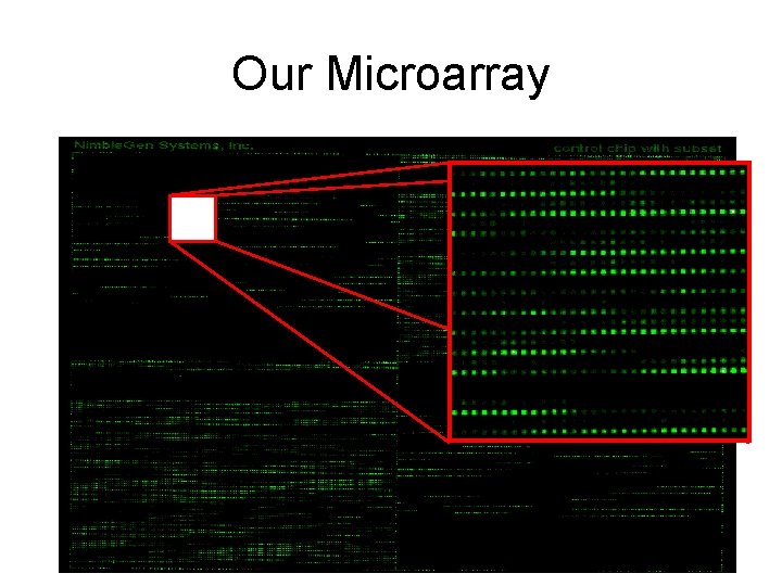
Our Microarray

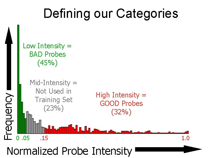
Defining our Categories Frequency Low Intensity = BAD Probes (45%) Mid-Intensity = Not Used in Training Set (23%) 0. 05 High Intensity = GOOD Probes (32%) . 15 Normalized Probe Intensity 1. 0

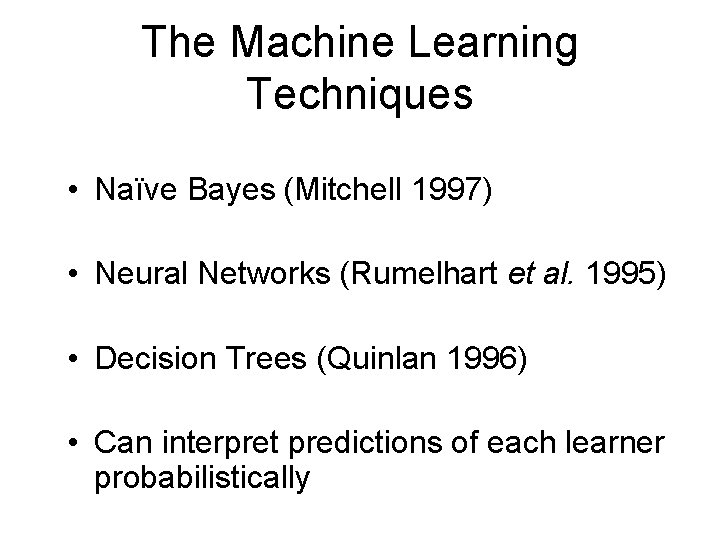
The Machine Learning Techniques • Naïve Bayes (Mitchell 1997) • Neural Networks (Rumelhart et al. 1995) • Decision Trees (Quinlan 1996) • Can interpret predictions of each learner probabilistically

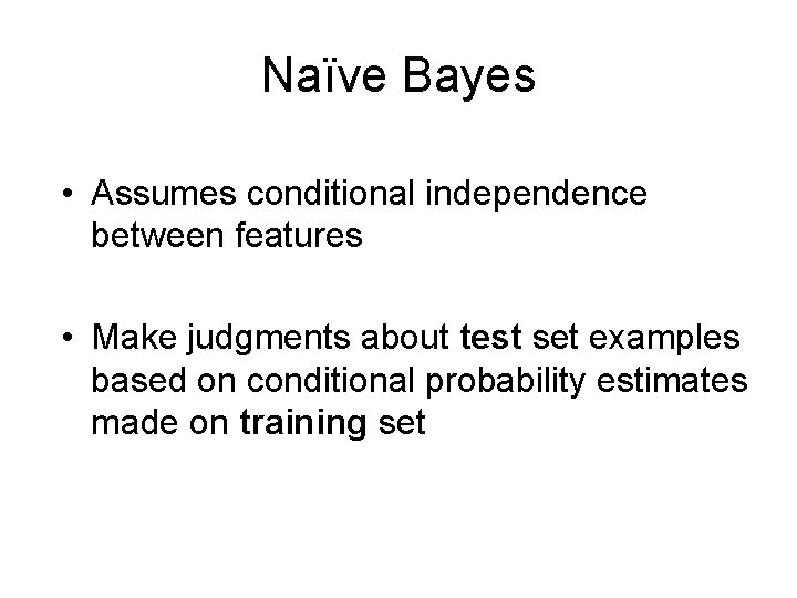
Naïve Bayes • Assumes conditional independence between features • Make judgments about test set examples based on conditional probability estimates made on training set

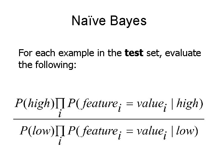
Naïve Bayes For each example in the test set, evaluate the following:

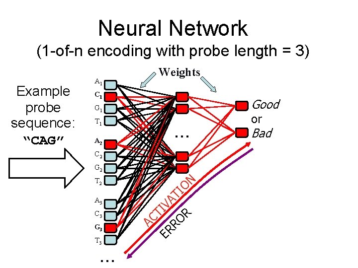
Neural Network (1 -of-n encoding with probe length = 3) A 1 C 1 Good G 1 T 1 … A 2 C 2 G 2 T 3 … R RO G 3 TI VA C 3 ER A 3 TI ON T 2 AC Example probe sequence: “CAG” Weights or Bad

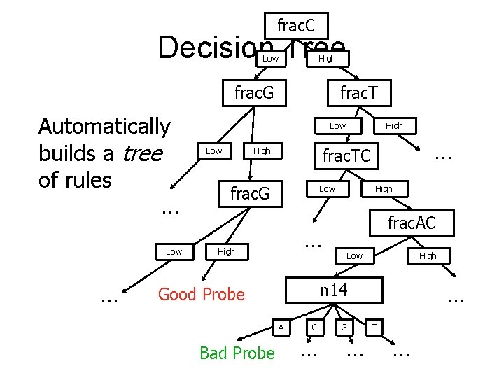
frac. C Decision Tree Low High frac. G Automatically builds a tree of rules … Low … frac. TC High frac. G Low High frac. AC … High Low High … n 14 Good Probe A Bad Probe High C … G … T …

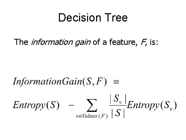
Decision Tree The information gain of a feature, F, is:

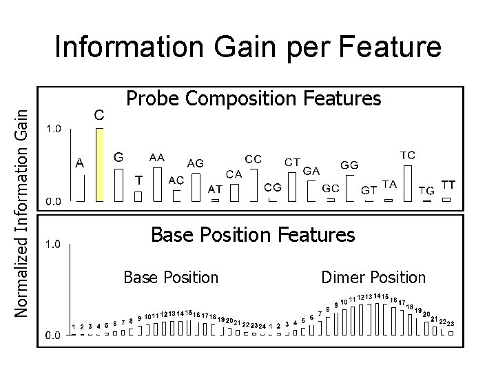
Normalized Information Gain per Feature Probe Composition Features Base Position Dimer Position

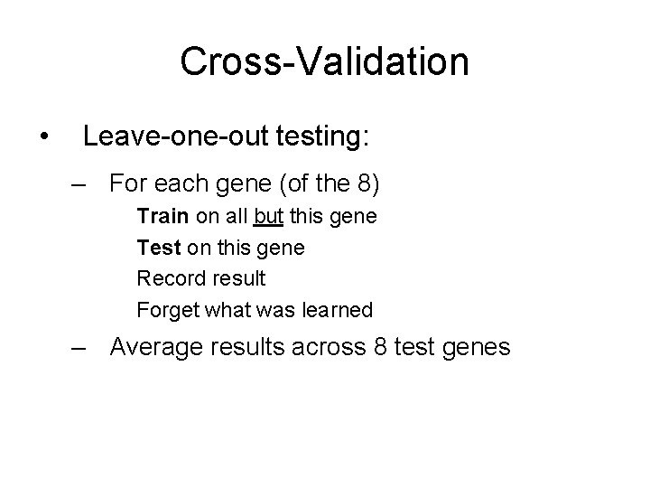
Cross-Validation • Leave-one-out testing: – For each gene (of the 8) Train on all but this gene Test on this gene Record result Forget what was learned – Average results across 8 test genes

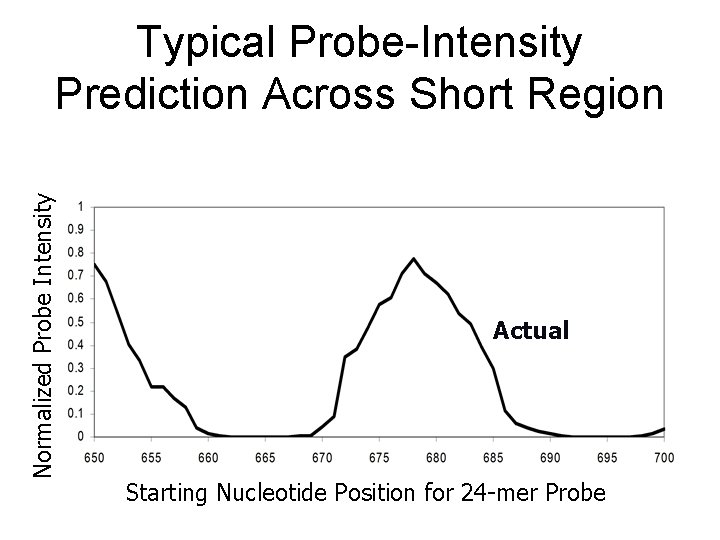
Normalized Probe Intensity Typical Probe-Intensity Prediction Across Short Region Actual Starting Nucleotide Position for 24 -mer Probe

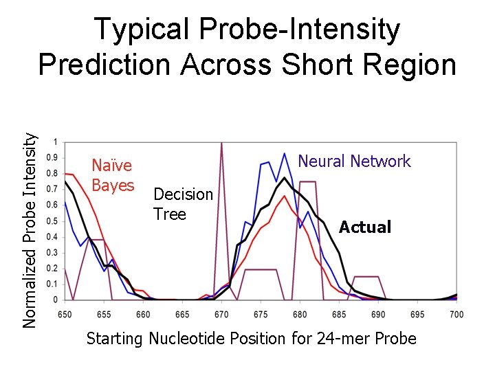
Normalized Probe Intensity Typical Probe-Intensity Prediction Across Short Region Naïve Bayes Neural Network Decision Tree Actual Starting Nucleotide Position for 24 -mer Probe

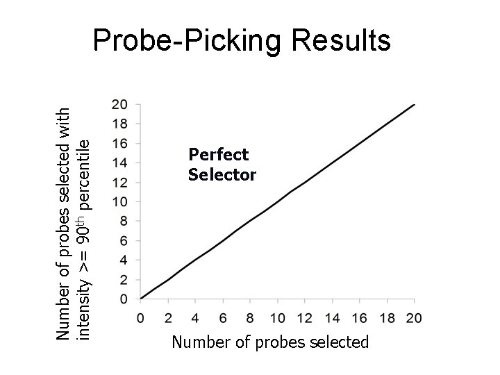
Number of probes selected with intensity >= 90 th percentile Probe-Picking Results Perfect Selector Number of probes selected

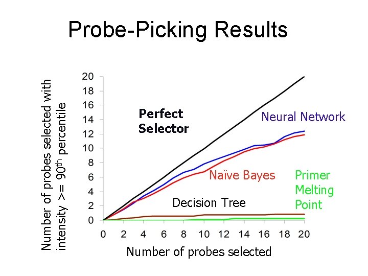
Number of probes selected with intensity >= 90 th percentile Probe-Picking Results Perfect Selector Neural Network Naïve Bayes Decision Tree Number of probes selected Primer Melting Point

A couple of final notes for the class:

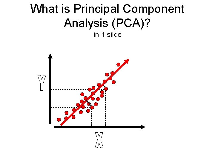
What is Principal Component Analysis (PCA)? in 1 silde

PCA Tutorial: • http: //csnet. otago. ac. nz/cosc 453/student_tutorials/principal_components. pdf

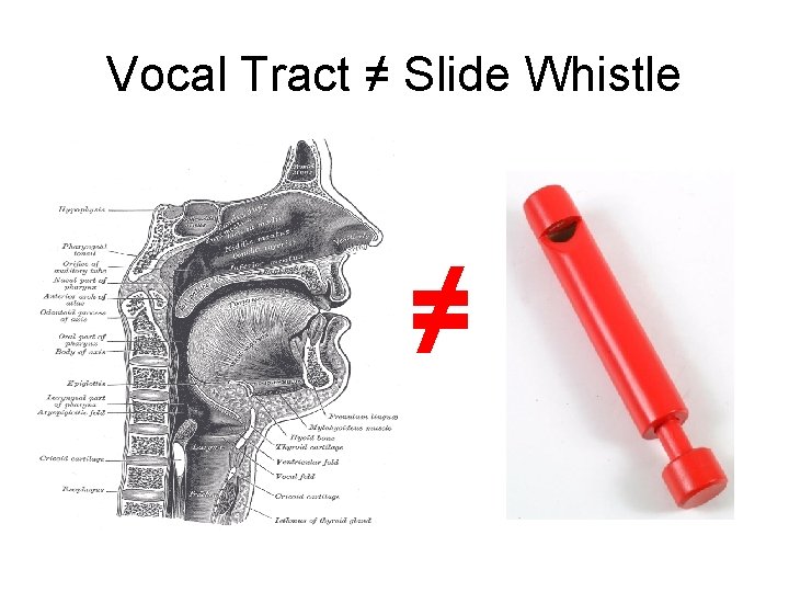
Vocal Tract ≠ Slide Whistle ≠