Lecture 6 Programming Paradigms and Algorithms WA 3

Lecture 6 -- Programming Paradigms and Algorithms W+A 3. 1, 3. 2, p. 178, 5. 1, 5. 3. 3, Chapter 6, 9. 2. 8, 10. 4. 1, Kumar 12. 1. 3 CSE 160/Berman

Common Parallel Programming Paradigms • • Embarrassingly parallel programs Workqueue Master/Slave programs Monte Carlo methods Regular, Iterative (Stencil) Computations Pipelined Computations Synchronous Computations CSE 160/Berman

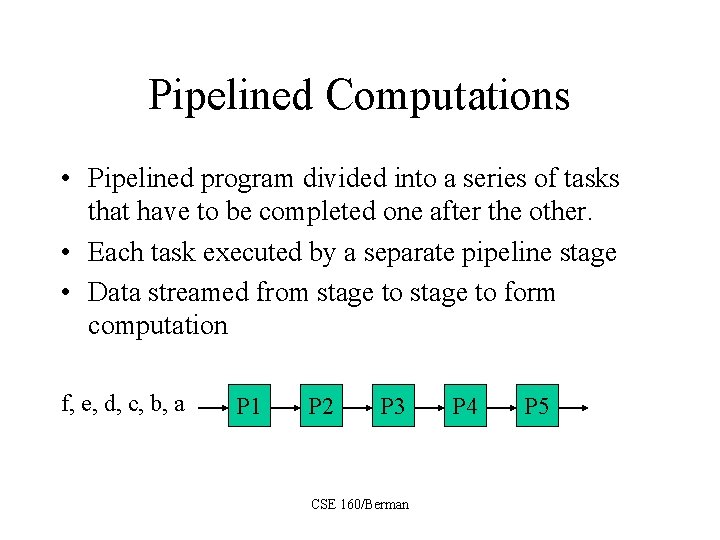
Pipelined Computations • Pipelined program divided into a series of tasks that have to be completed one after the other. • Each task executed by a separate pipeline stage • Data streamed from stage to form computation f, e, d, c, b, a P 1 P 2 P 3 CSE 160/Berman P 4 P 5

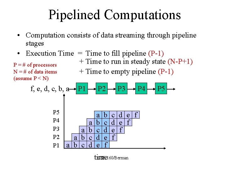
Pipelined Computations • Computation consists of data streaming through pipeline stages • Execution Time = Time to fill pipeline (P-1) + Time to run in steady state (N-P+1) P = # of processors N = # of data items + Time to empty pipeline (P-1) (assume P < N) f, e, d, c, b, a P 5 P 4 P 3 P 2 P 1 a a b c d P 2 a b c d e f P 3 c d e f e f f CSE 160/Berman time P 4 P 5

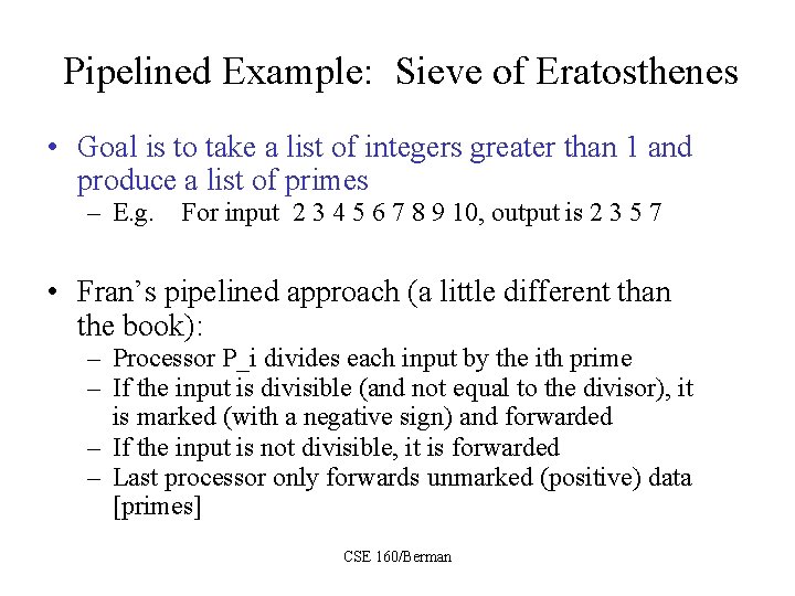
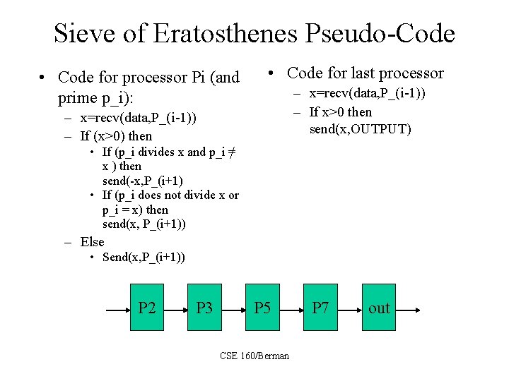
Pipelined Example: Sieve of Eratosthenes • Goal is to take a list of integers greater than 1 and produce a list of primes – E. g. For input 2 3 4 5 6 7 8 9 10, output is 2 3 5 7 • Fran’s pipelined approach (a little different than the book): – Processor P_i divides each input by the ith prime – If the input is divisible (and not equal to the divisor), it is marked (with a negative sign) and forwarded – If the input is not divisible, it is forwarded – Last processor only forwards unmarked (positive) data [primes] CSE 160/Berman

Sieve of Eratosthenes Pseudo-Code • Code for processor Pi (and prime p_i): • Code for last processor – x=recv(data, P_(i-1)) – If x>0 then send(x, OUTPUT) – x=recv(data, P_(i-1)) – If (x>0) then • If (p_i divides x and p_i =/ x ) then send(-x, P_(i+1) • If (p_i does not divide x or p_i = x) then send(x, P_(i+1)) – Else • Send(x, P_(i+1)) P 2 P 3 P 5 CSE 160/Berman P 7 out

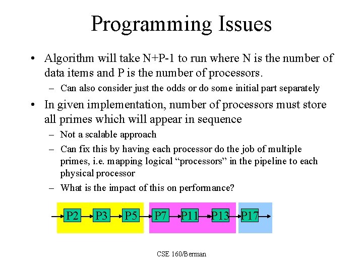
Programming Issues • Algorithm will take N+P-1 to run where N is the number of data items and P is the number of processors. – Can also consider just the odds or do some initial part separately • In given implementation, number of processors must store all primes which will appear in sequence – Not a scalable approach – Can fix this by having each processor do the job of multiple primes, i. e. mapping logical “processors” in the pipeline to each physical processor – What is the impact of this on performance? P 2 P 3 P 5 P 7 P 11 P 13 P 17 CSE 160/Berman

More Programming Issues • In pipelined algorithm, flow of data moves through processors in lockstep, attempt to balance work so that there is no bottleneck at any processor • In mid-80’s, processors developed to support in hardware this kind of parallel pipelined computation • Two commercial products from Intel: Warp (1 D array) and i. Warp (components for 2 D array) • Warp and i. Warp were meant to operate synchronously Wavefront Array Processor (S. Y. Kung) was meant to operate asynchronously, i. e. arrival of data would signal that it was time to execute CSE 160/Berman

Systolic Arrays • Warp and i. Warp were examples of systolic arrays – Systolic means regular and rhythmic, data was supposed to move through pipelined computational units in a regular and rhythmic fashion • Systolic arrays meant to be special-purpose processors or co-processors and were very finegrained – Processors implement a limited and very simple computation, usually called cells – Communication is very fast, granularity meant to be around 1! CSE 160/Berman

Systolic Algorithms • Systolic arrays built to support systolic algorithms, a hot area of research in the early 80’s • Systolic algorithms used pipelining through various kinds of arrays to accomplish computational goals – Some of the data streaming and applications were very creative and quite complex – CMU a hotbed of systolic algorithm and array research (especially H. T. Kung and his group) CSE 160/Berman

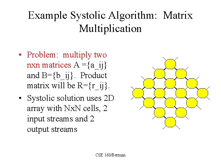
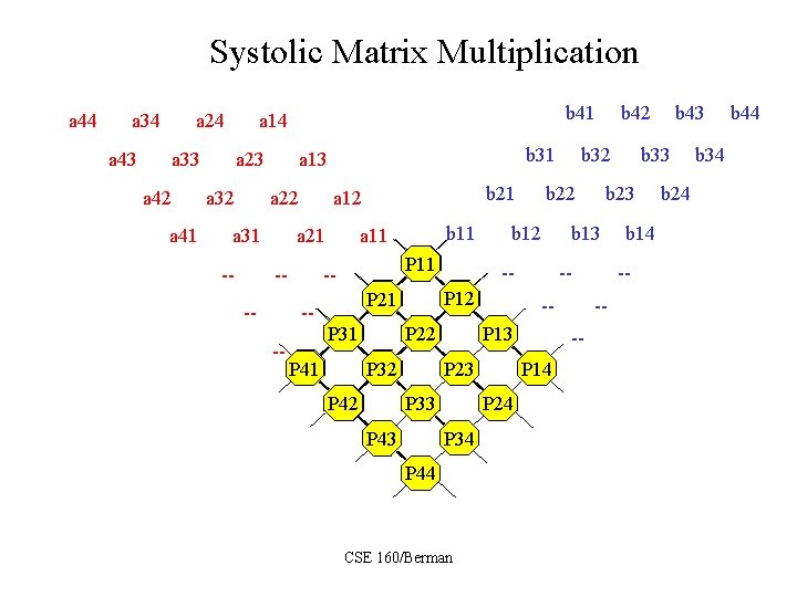
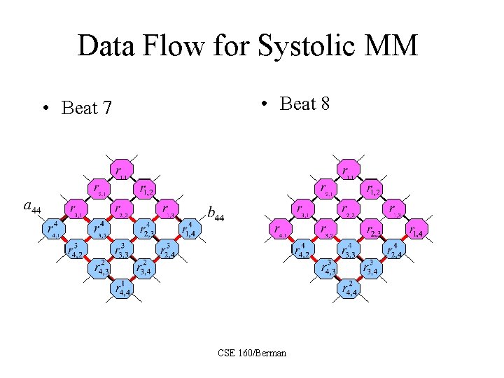
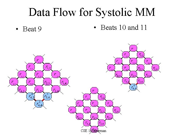
Example Systolic Algorithm: Matrix Multiplication • Problem: multiply two nxn matrices A ={a_ij} and B={b_ij}. Product matrix will be R={r_ij}. • Systolic solution uses 2 D array with Nx. N cells, 2 input streams and 2 output streams CSE 160/Berman

Systolic Matrix Multiplication a 44 a 34 a 24 a 43 a 14 == a 33 a 42 a 41 a 23 a 32 a 13 == a 22 a 31 -- == --- b 21 b 11 a 11 P 11 -- P 32 P 41 -P 13 P 24 P 34 P 43 P 44 CSE 160/Berman b 14 -- --- P 14 P 23 P 33 P 42 -- b 43 b 33 b 23 b 13 -- P 22 b 42 b 32 b 22 b 12 P 21 P 31 b 31 == a 12 === a 21 b 41 == b 24 b 34 b 44

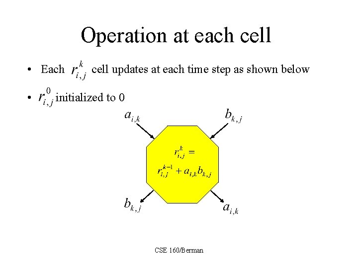
Operation at each cell • Each • cell updates at each time step as shown below initialized to 0 CSE 160/Berman

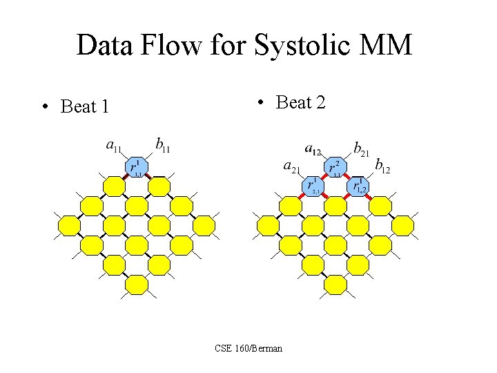
Data Flow for Systolic MM • Beat 1 • Beat 2 CSE 160/Berman

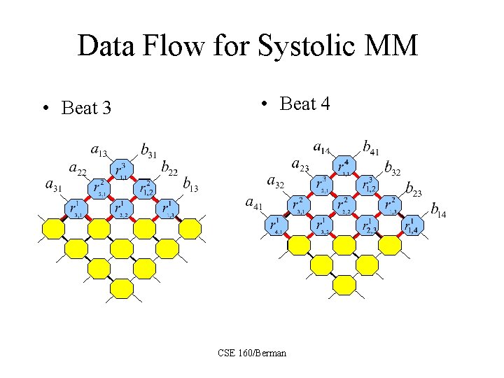
Data Flow for Systolic MM • Beat 3 • Beat 4 CSE 160/Berman

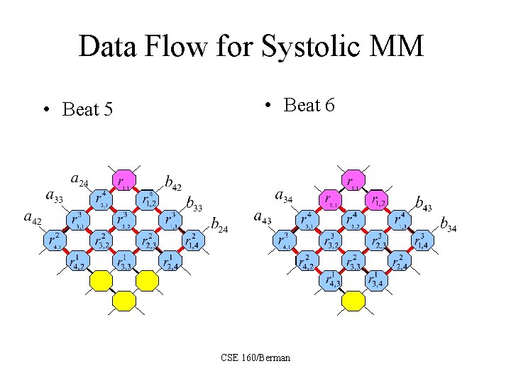
Data Flow for Systolic MM • Beat 5 • Beat 6 CSE 160/Berman

Data Flow for Systolic MM • Beat 7 • Beat 8 CSE 160/Berman

Data Flow for Systolic MM • Beat 9 • Beats 10 and 11 CSE 160/Berman

Programming Issues • Performance of systolic algorithms based on fine granularity (1 update about the same as a communication) and regular dataflow – Can be done on asynchronous platforms with tagging but must ensure that idle time does not dominate computation • Many systolic algorithms do not map well to more general MIMD or distributed platforms CSE 160/Berman

Synchronous Computations • Synchronous computations have the form (Barrier) Computation Barrier Computation … • Frequency of the barrier and homogeneity of the intervening computations on the processors may vary • We’ve seen some synchronous computations already (Jacobi 2 D, Systolic MM) CSE 160/Berman

Synchronous Computations • Synchronous computations can be simulated using asynchronous programming models – Iterations can be tagged so that the appropriate data is combined • Performance of such computations depends on the granularity of the platform, how expensive synchronizations are, and how much time is spent idle waiting for the right data to arrive CSE 160/Berman

Barrier Synchronizations • Barrier synchronizations can be implemented in many ways: – As part of the algorithm – As a part of the communication library • PVM and MPI have barrier operations – In hardware • Implementations vary CSE 160/Berman

Review • What is time balancing? How do we use time-balancing to decompose Jacobi 2 D for a cluster? • Describe the general flow of data and computation in a pipelined algorithm. What are possible bottlenecks? • What are three stages of a pipelined program? How long will each take with P processors and N data items? • Would pipelined programs be well supported by SIMD machines? Why or why not? • What is a systolic program? Would a systolic program be efficiently supported on a general-purpose MPP? Why or why not? CSE 160/Berman

Common Parallel Programming Paradigms • • Embarrassingly parallel programs Workqueue Master/Slave programs Monte Carlo methods Regular, Iterative (Stencil) Computations Pipelined Computations Synchronous Computations CSE 160/Berman

Synchronous Computations • Synchronous computations are programs structured as a group of separate computations which must at times wait for each other before proceeding • Fully synchronous computations = programs in which all processes synchronized at regular points • Computation between synchronizations often called stages CSE 160/Berman

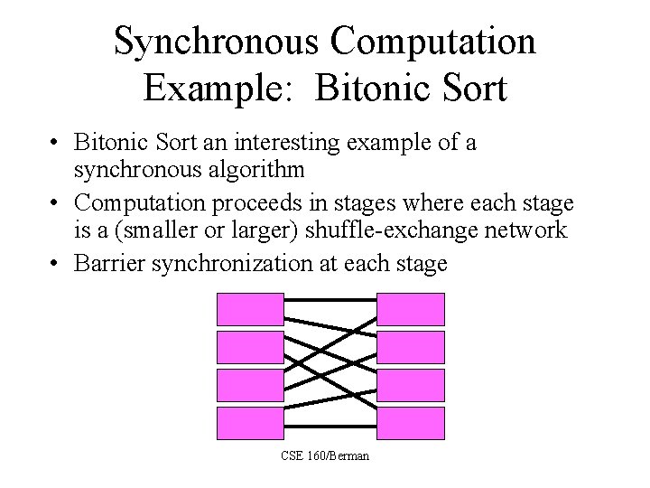
Synchronous Computation Example: Bitonic Sort • Bitonic Sort an interesting example of a synchronous algorithm • Computation proceeds in stages where each stage is a (smaller or larger) shuffle-exchange network • Barrier synchronization at each stage CSE 160/Berman

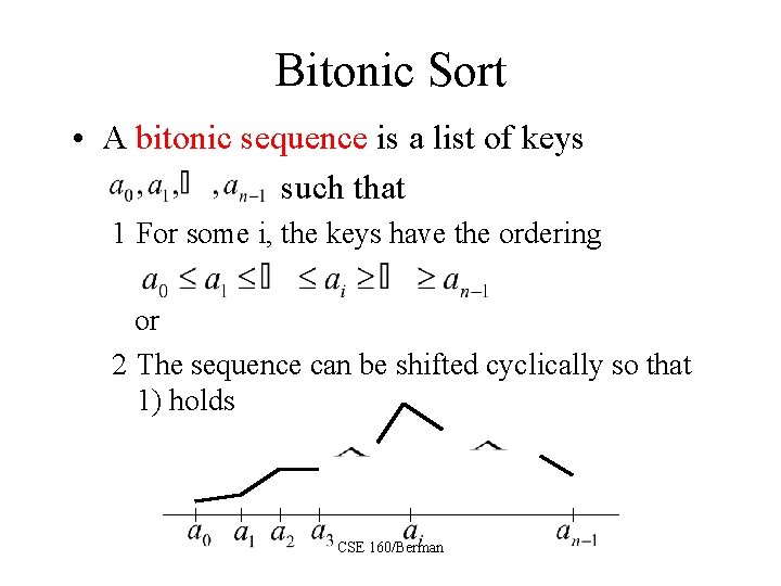
Bitonic Sort • A bitonic sequence is a list of keys such that 1 For some i, the keys have the ordering or 2 The sequence can be shifted cyclically so that 1) holds CSE 160/Berman

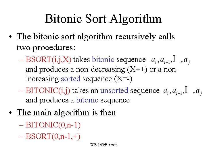
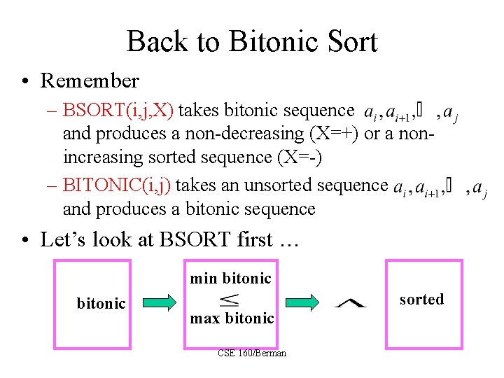
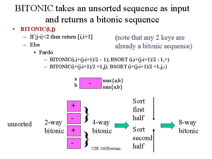
Bitonic Sort Algorithm • The bitonic sort algorithm recursively calls two procedures: – BSORT(i, j, X) takes bitonic sequence and produces a non-decreasing (X=+) or a nonincreasing sorted sequence (X=-) – BITONIC(i, j) takes an unsorted sequence and produces a bitonic sequence • The main algorithm is then – BITONIC(0, n-1) – BSORT(0, n-1, +) CSE 160/Berman

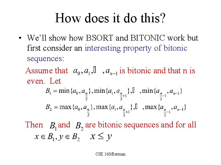
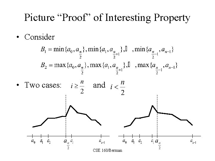
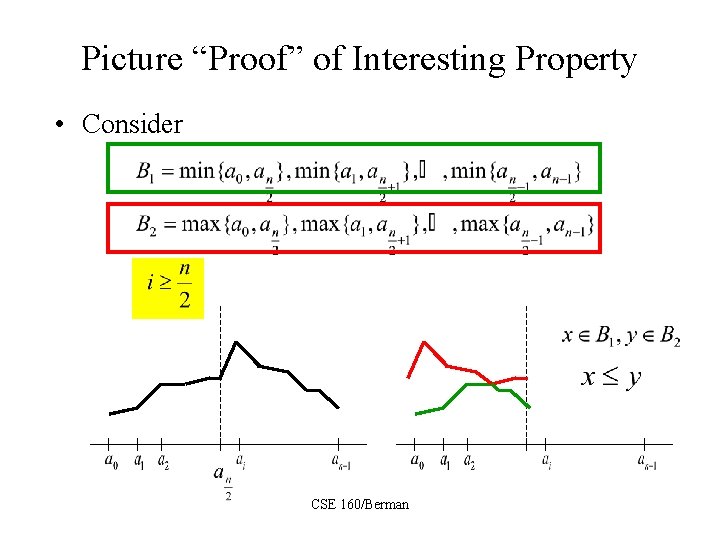
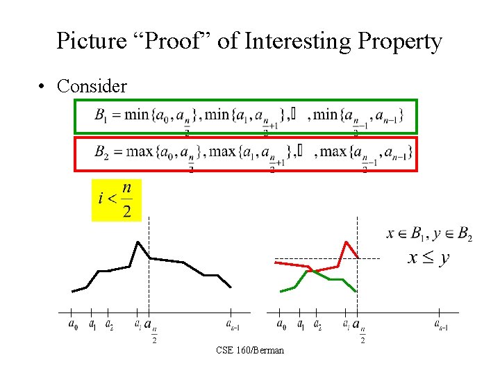
How does it do this? • We’ll show BSORT and BITONIC work but first consider an interesting property of bitonic sequences: Assume that is bitonic and that n is even. Let Then and are bitonic sequences and for all CSE 160/Berman

Picture “Proof” of Interesting Property • Consider • Two cases: and CSE 160/Berman

Picture “Proof” of Interesting Property • Consider CSE 160/Berman

Picture “Proof” of Interesting Property • Consider CSE 160/Berman

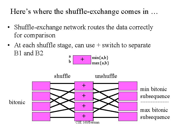
Back to Bitonic Sort • Remember – BSORT(i, j, X) takes bitonic sequence and produces a non-decreasing (X=+) or a nonincreasing sorted sequence (X=-) – BITONIC(i, j) takes an unsorted sequence and produces a bitonic sequence • Let’s look at BSORT first … min bitonic sorted max bitonic CSE 160/Berman

Here’s where the shuffle-exchange comes in … • Shuffle-exchange network routes the data correctly for comparison • At each shuffle stage, can use + switch to separate B 1 and B 2 a min{a, b} + b max{a, b} shuffle unshuffle + bitonic + + + CSE 160/Berman min bitonic subsequence max bitonic subsequence

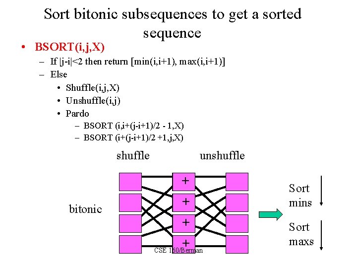
Sort bitonic subsequences to get a sorted sequence • BSORT(i, j, X) – If |j-i|<2 then return [min(i, i+1), max(i, i+1)] – Else • Shuffle(i, j, X) • Unshuffle(i, j) • Pardo – BSORT (i, i+(j-i+1)/2 - 1, X) – BSORT (i+(j-i+1)/2 +1, j, X) shuffle unshuffle + bitonic + + + CSE 160/Berman Sort mins Sort maxs

BITONIC takes an unsorted sequence as input and returns a bitonic sequence • BITONIC(i, j) – If |j-i|<2 then return [i, i+1] – Else • Pardo (note that any 2 keys are already a bitonic sequence) – BITONIC(i, i+(j-i+1)/2 – 1); BSORT (i, i+(j-i+1)/2 - 1, +) – BITONIC(i+(j-i+1)/2 +1, j); BSORT (i+(j-i+1)/2 +1, j, -) a b unsorted + 2 -way bitonic + - - } } max{a, b} min{a, b} 4 -way bitonic CSE 160/Berman Sort first half Sort second half 8 -way bitonic

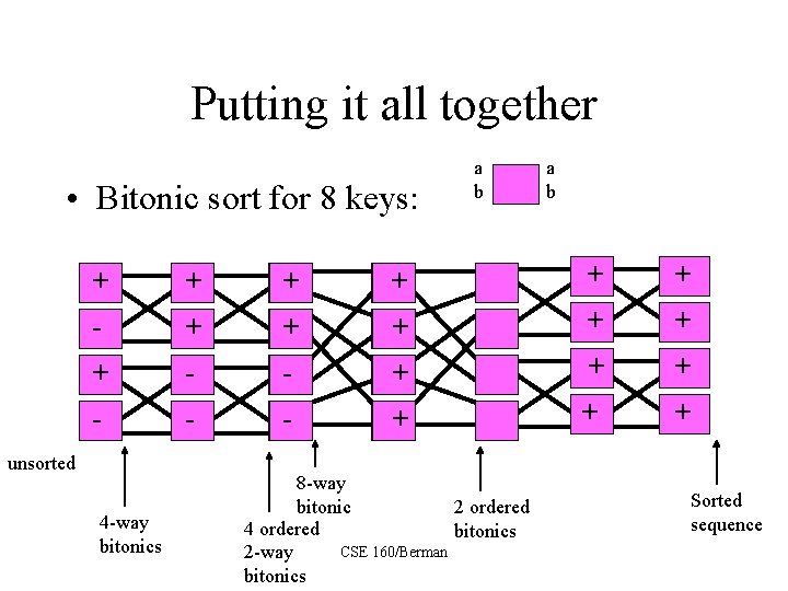
Putting it all together • Bitonic sort for 8 keys: a b + + + + - + - + + + + unsorted 4 -way bitonics 8 -way bitonic 2 ordered 4 ordered bitonics CSE 160/Berman 2 -way bitonics + + Sorted sequence

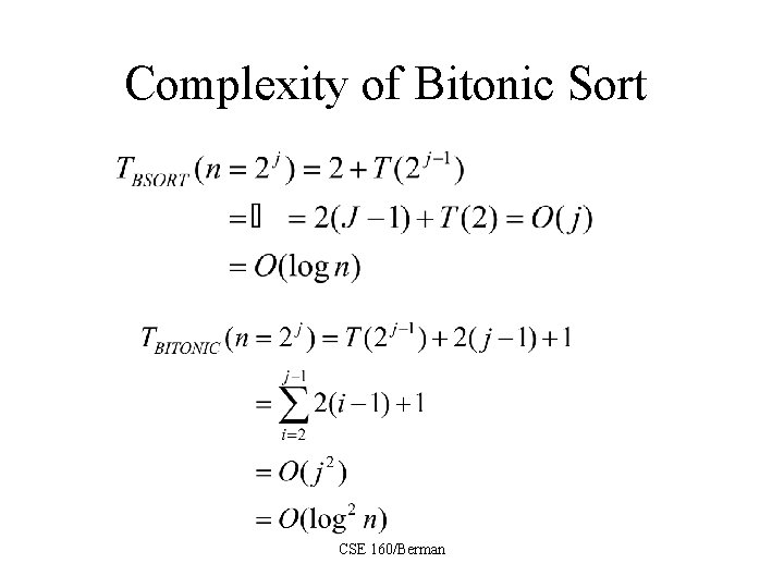
Complexity of Bitonic Sort CSE 160/Berman

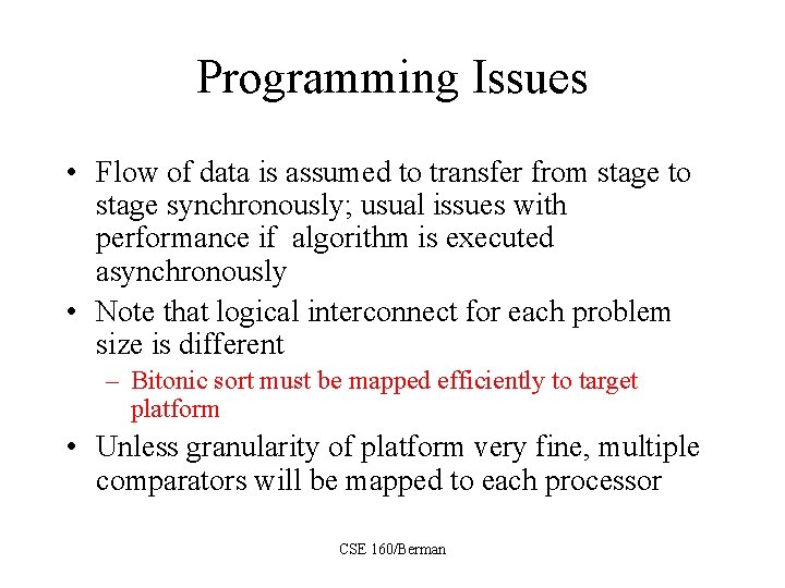
Programming Issues • Flow of data is assumed to transfer from stage to stage synchronously; usual issues with performance if algorithm is executed asynchronously • Note that logical interconnect for each problem size is different – Bitonic sort must be mapped efficiently to target platform • Unless granularity of platform very fine, multiple comparators will be mapped to each processor CSE 160/Berman

Review • What is a a synchronous computation? What is a fully synchronous computation? • What is a bitonic sequence? • What do the procedures BSORT and BITONIC do? • How would you implement Bitonic Sort in a performance-efficient way? CSE 160/Berman

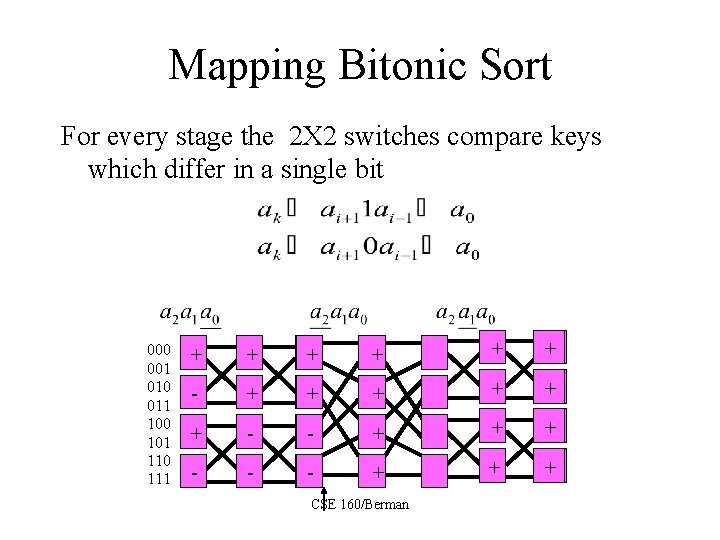
Mapping Bitonic Sort For every stage the 2 X 2 switches compare keys which differ in a single bit 000 001 010 011 100 101 110 111 + + + - - + + + - - - + + + CSE 160/Berman

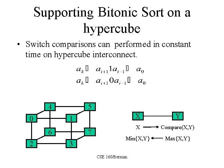
Supporting Bitonic Sort on a hypercube • Switch comparisons can performed in constant time on hypercube interconnect. 4 0 5 6 2 X Y X Compare(X, Y) Min{X, Y} Max{X, Y} 1 7 3 CSE 160/Berman

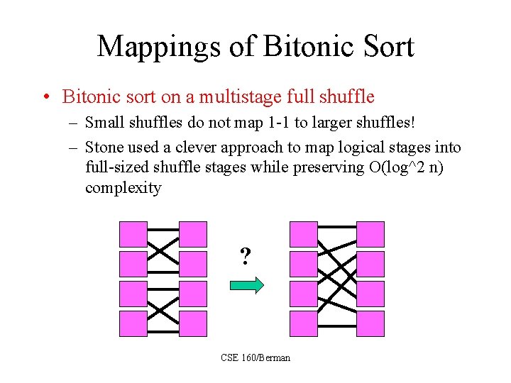
Mappings of Bitonic Sort • Bitonic sort on a multistage full shuffle – Small shuffles do not map 1 -1 to larger shuffles! – Stone used a clever approach to map logical stages into full-sized shuffle stages while preserving O(log^2 n) complexity ? CSE 160/Berman

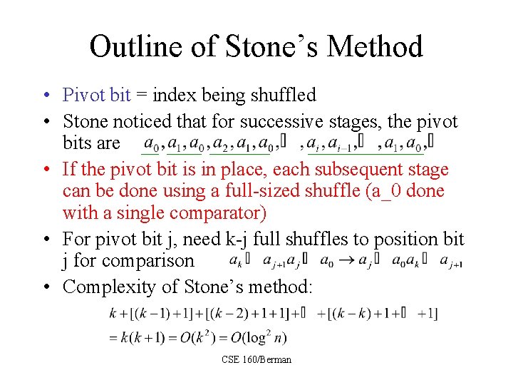
Outline of Stone’s Method • Pivot bit = index being shuffled • Stone noticed that for successive stages, the pivot bits are • If the pivot bit is in place, each subsequent stage can be done using a full-sized shuffle (a_0 done with a single comparator) • For pivot bit j, need k-j full shuffles to position bit j for comparison • Complexity of Stone’s method: CSE 160/Berman

Many-one Mappings of Bitonic Sort • For platforms where granularity is coarser, it will be more cost-efficient to map multiple comparators to one processor • Several possible conventional mappings - - - + + + - - + • Compare-split provides another approach … CSE 160/Berman + + -

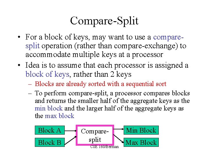
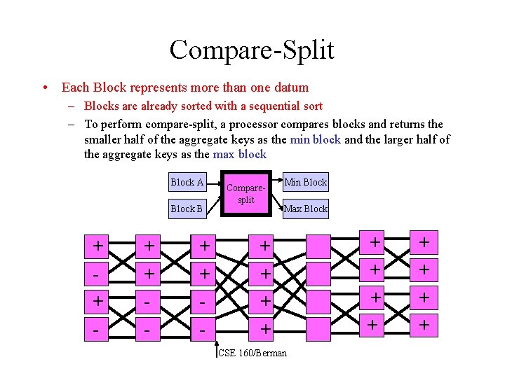
Compare-Split • For a block of keys, may want to use a comparesplit operation (rather than compare-exchange) to accommodate multiple keys at a processor • Idea is to assume that each processor is assigned a block of keys, rather than 2 keys – Blocks are already sorted with a sequential sort – To perform compare-split, a processor compares blocks and returns the smaller half of the aggregate keys as the min block and the larger half of the aggregate keys as the max block Block A Block B Comparesplit CSE 160/Berman Min Block Max Block

Compare-Split • Each Block represents more than one datum – Blocks are already sorted with a sequential sort – To perform compare-split, a processor compares blocks and returns the smaller half of the aggregate keys as the min block and the larger half of the aggregate keys as the max block Block A Block B + + - Comparesplit Min Block Max Block + + CSE 160/Berman + + + +

Performance Issues • What is the complexity of compare-split? • How do we optimize compare-split? – How many datum per block? – How to allocate blocks per processors? – How to synchronize intra-block sorting with inter-block communication? CSE 160/Berman